|
|
|
|
1
|
|
2
|
|
3
|
Click Add.
|
|
4
|
|
5
|
Click Add.
|
|
6
|
Click
|
|
7
|
|
8
|
Click
|
|
1
|
|
2
|
Browse to the model’s Application Libraries folder and double-click the file heat_exchanger_plate_geom_sequence.mph.
|
|
3
|
|
1
|
|
2
|
|
3
|
|
4
|
|
5
|
|
1
|
|
2
|
|
3
|
|
1
|
In the Model Builder window, expand the Component 1 (comp1)>Definitions node, then click Component 1 (comp1)>Pipe Flow (pfl).
|
|
2
|
|
3
|
|
1
|
|
2
|
|
3
|
From the list, choose Square.
|
|
4
|
|
1
|
|
1
|
|
3
|
|
4
|
|
5
|
|
1
|
|
3
|
|
4
|
|
1
|
|
2
|
|
3
|
|
4
|
|
1
|
|
2
|
|
1
|
|
2
|
|
3
|
|
4
|
|
1
|
|
2
|
|
3
|
|
4
|
|
1
|
|
2
|
|
1
|
|
2
|
|
3
|
|
4
|
|
5
|
|
6
|
|
7
|
|
8
|
|
9
|
|
10
|
|
11
|
|
12
|
|
1
|
|
2
|
|
1
|
|
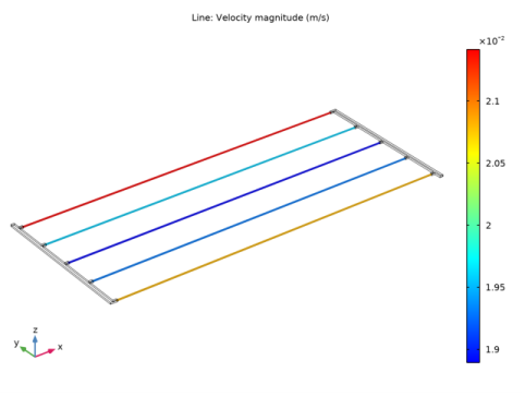
2
|
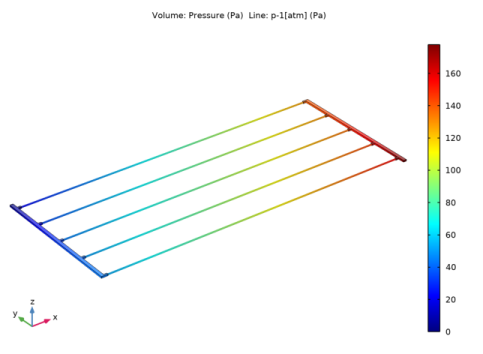
In the Settings window for Line, click Replace Expression in the upper-right corner of the Expression section. From the menu, choose Component 1 (comp1)>Pipe Flow>pfl.U - Velocity magnitude - m/s.
|
|
3
|
Click to expand the Range section. Locate the Coloring and Style section. Select the Color legend check box.
|
|
4
|
|
1
|
|
2
|
|
1
|
|
2
|
|
1
|
|
2
|
|
3
|
|
1
|
|
2
|
|
3
|
|
1
|
|
2
|
|
3
|
|
4
|
|
5
|
|
6
|
|
7
|
|
8
|
|
9
|
|
1
|
|
2
|
Select the object wp1 only.
|
|
3
|
|
4
|
|
5
|
|
6
|
Locate the Selections of Resulting Entities section. Select the Resulting objects selection check box.
|
|
7
|
|
1
|
|
2
|
|
3
|
|
4
|
|
5
|
|
6
|
|
1
|
|
2
|
|
3
|
|
4
|
|
1
|
|
2
|
|
3
|
|
4
|
|
5
|
|
6
|
|
1
|
In the Model Builder window, under Component 1 (comp1)>Geometry 1 right-click Block 2 (blk2) and choose Duplicate.
|
|
2
|
|
3
|
|
4
|
|
5
|
|
1
|
|
2
|
|
3
|
|
4
|
|
5
|
|
1
|
|
2
|
On the object fin, select Domains 1–12 only.
|
|
3
|