PDF

Ground Heat Recovery for Radiant Floor Heating
Introduction
Geothermal heating is an environmentally friendly and energy efficient method to supply modern and well insulated houses with heat. The investment costs are higher than for gas or oil heating so there is a need to investigate the possibilities of arranging heat collectors in the subsurface.
Figure 1: Example of heat recovery coils in a garden, connected to a dwelling via a heat pump.
This example compares three different patterns embedded in the subsurface. Typical thermal properties of an uppermost soil layer in a garden are used for the calculations.
Figure 2: Patterns for the heat collectors.
Model Definition
The three patterns for the pipe arrangement are shown in Figure 2. The geometry subsequence functionality in COMSOL Multiphysics offers the possibility to perform the analysis over different pipe arrangements within the same model using a parametric sweep.
This model uses functions and events to describe the real operating conditions. For the subsurface, a temperature gradient with depth is prescribed. At the surface, a time dependent temperature is applied which corresponds to typical temperature variations in central Europe.
Assuming that the fluid properties are temperature-independent, the inlet temperature of the heat collector required to reach a certain heat extraction rate, P(t) is given by
(1)
where ρ and Cp the density and specific heat capacity for the fluid inside the pipes and the volumetric flow rate, here equal to 1 l/s.
The dynamic heat extraction is triggered according to a typical daily heat demand of a single-family house. The heat extraction process is active each day until the demanded heat is extracted. When the demand is reached, the heat extraction is stopped but the fluid flow in the pipes still continue at a lower rate. In this application, this flow rate during inaction of the pump is set to 1/10th of the operating flow rate, that is, 0.1 l/s.
Results and Discussion
The pipe temperature for the third pattern after two days is shown below.
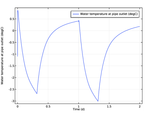
Figure 3 shows the outlet temperature over time for the third pattern. It is important to make sure that the fluid inside the pipes stays above a certain value. In this example, water is used as working fluid. However, during winter, the ambient temperature above the surface may reach values below 0 °C. In practical situations, antifreezes — such as glycerol — are added to water and this application assumes that such additives do not modify its thermal properties.
Figure 3: Outlet temperatures for the third pattern.
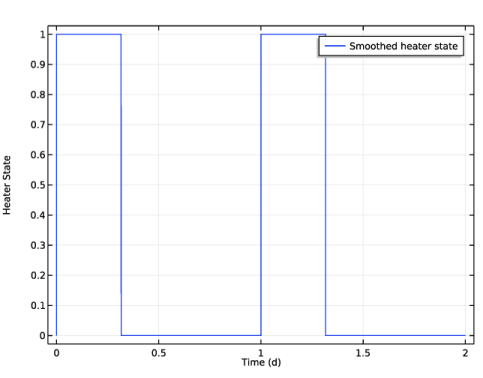
The temperature variations in Figure 3 correspond to the moments when the heater is turned on or off. The graph of the heater state in time is shown in Figure 4.
Figure 4: Heater state in time for the third pattern. A value of 0 indicates that the heater is turned off while 1 indicates that the heater is turned on.
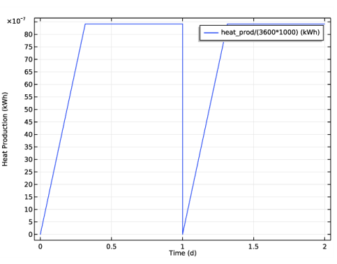
The heater state itself depends on the daily heat production. As soon as the heat production reaches the daily demand, the heater state is turned off until the next day. Figure 5 shows the heat production the two days of simulation time. Just after the daily requirement of 30 kWh, the production is stopped until the next day.
Figure 5: Heat production for the third pattern.
Notes About the COMSOL Implementation
This model uses several interpolation functions, which are based on rough estimations and local temperature variations, which may differ for your case. The functions needs to be replaced by your own measured data. Then, you need to make sure that the time stepping is still fine enough to resolve them.
Application Library path: Pipe_Flow_Module/Heat_Transfer/ground_heat_recovery
Modeling Instructions
From the File menu, choose New.
New
In the New window, click Model Wizard.
Model Wizard
1
In the Model Wizard window, click 3D.
2
In the Select Physics tree, select Heat Transfer>Heat Transfer in Solids (ht).
3
Click Add.
4
In the Select Physics tree, select Heat Transfer>Heat Transfer in Pipes (htp).
5
Click Add.
6
In the Select Physics tree, select Mathematics>ODE and DAE Interfaces>Events (ev).
7
Click Add.
8
In the Select Physics tree, select Mathematics>ODE and DAE Interfaces>Global ODEs and DAEs (ge).
9
Click Add.
10
Click Study.
11
In the Select Study tree, select General Studies>Time Dependent.
12
Click Done.
Geometry 1
This example demonstrates how to use part import and programming to perform the simulation for different geometries. Start by importing the parts from a file, as shown below.
1
In the Geometry toolbar, click Parts and choose Load Part.
2
3
In the Load Part dialog box, in the Select parts list, choose Pattern 1, Pattern 2, and Pattern 3.
4
Global Definitions
Parameters 1
Define the parameter that will be used to call the different patterns.
1
In the Model Builder window, under Global Definitions click Parameters 1.
2
In the Settings window for Parameters, locate the Parameters section.
3
This parameter is now used to import the different patterns into the work plane based on a logical expression.
Add the remaining parameters.
4
Geometry 1
Work Plane 1 (wp1)
1
In the Geometry toolbar, click Work Plane.
2
In the Settings window for Work Plane, locate the Plane Definition section.
3
In the z-coordinate text field, type -depth.
4
Locate the Selections of Resulting Entities section. Find the Cumulative selection subsection. Click New.
5
In the New Cumulative Selection dialog box, type Pipes in the Name text field.
6
The above step ensures that, independently of the pattern you choose, the pipes are selected correctly.
Work Plane 1 (wp1)>Plane Geometry
Right-click Work Plane 1 (wp1) and choose Show Work Plane.
Work Plane 1 (wp1)>If 1 (if1)
1
In the Work Plane toolbar, click Programming and choose If + End If.
2
In the Settings window for If, locate the If section.
3
In the Condition text field, type pattern==1.
Work Plane 1 (wp1)>Import 1 (imp1)
1
In the Work Plane toolbar, click Import.
2
In the Settings window for Import, locate the Import section.
3
From the Source list, choose Geometry sequence.
4
From the Geometry list, choose Pattern 1.
Work Plane 1 (wp1)>Else If 1 (elseif1)
1
In the Model Builder window, right-click Plane Geometry and choose Programming>Else If.
2
In the Settings window for Else If, locate the Else If section.
3
In the Condition text field, type pattern==2.
Work Plane 1 (wp1)>Import 2 (imp2)
1
In the Work Plane toolbar, click Import.
2
In the Settings window for Import, locate the Import section.
3
From the Source list, choose Geometry sequence.
4
From the Geometry list, choose Pattern 2.
Work Plane 1 (wp1)>Else 1 (else1)
Right-click Plane Geometry and choose Programming>Else.
Work Plane 1 (wp1)>Import 3 (imp3)
1
In the Work Plane toolbar, click Import.
2
In the Settings window for Import, locate the Import section.
3
From the Source list, choose Geometry sequence.
4
From the Geometry list, choose Pattern 3.
5
In the Model Builder window, click Geometry 1.
Polygon 1 (pol1)
1
In the Geometry toolbar, click More Primitives and choose Polygon.
2
In the Settings window for Polygon, locate the Coordinates section.
3
4
Locate the Selections of Resulting Entities section. Find the Cumulative selection subsection. From the Contribute to list, choose Pipes.
Copy 1 (copy1)
1
In the Geometry toolbar, click Transforms and choose Copy.
2
3
In the Settings window for Copy, locate the Displacement section.
4
In the x text field, type 0.5.
5
Locate the Selections of Resulting Entities section. Find the Cumulative selection subsection. From the Contribute to list, choose Pipes.
Block 1 (blk1)
1
In the Geometry toolbar, click Block.
2
In the Settings window for Block, locate the Size and Shape section.
3
In the Width text field, type 15.
4
In the Depth text field, type 22.
5
In the Height text field, type depth+3[m].
6
Locate the Position section. In the z text field, type -(depth+3[m]).
7
Locate the Selections of Resulting Entities section. Find the Cumulative selection subsection. Click New.
8
In the New Cumulative Selection dialog box, type Ground in the Name text field.
9
10
Right-click Block 1 (blk1) and choose Build All Objects.
11
Click the Zoom Extents button in the Graphics toolbar.
Definitions
Hide for Physics 1
1
In the Model Builder window, expand the Component 1 (comp1)>Definitions node.
2
Right-click View 1 and choose Hide for Physics.
3
In the Settings window for Hide for Physics, locate the Geometric Entity Selection section.
4
From the Geometric entity level list, choose Boundary.
5
Global Definitions
Define the functions for the surface temperature and the initial temperature.
Yearly Temperature Profile
1
In the Home toolbar, click Functions and choose Global>Interpolation.
2
In the Settings window for Interpolation, type Yearly Temperature Profile in the Label text field.
3
Locate the Definition section. In the Function name text field, type T_z0.
4
Click Load from File.
5
6
Locate the Interpolation and Extrapolation section. From the Interpolation list, choose Piecewise cubic.
7
Locate the Units section. In the Arguments text field, type a.
8
In the Function text field, type degC.
9
Click Create Plot.
Results
Temperature Profile
1
In the Settings window for 1D Plot Group, type Temperature Profile in the Label text field.
2
Click to expand the Title section. From the Title type list, choose None.
3
Locate the Plot Settings section. In the x-axis label text field, type Month.
Line Graph 1
1
In the Model Builder window, expand the Temperature Profile node, then click Line Graph 1.
2
In the Settings window for Line Graph, locate the y-Axis Data section.
3
In the Expression text field, type T_z0(root.t[a])[1/degC].
4
Locate the x-Axis Data section. In the Expression text field, type root.t*12.
5
Select the Description check box.
6
7
Click to expand the Coloring and Style section. In the Width text field, type 3.
Point Graph 1
1
In the Model Builder window, click Point Graph 1.
2
In the Settings window for Point Graph, locate the y-Axis Data section.
3
In the Expression text field, type T_z0(root.t[a])[1/degC].
4
Locate the x-Axis Data section. In the Expression text field, type root.t*12.
5
Click to expand the Coloring and Style section. In the Width text field, type 3.
Left Extrapolation
1
In the Model Builder window, click Left Extrapolation.
2
In the Settings window for Line Graph, locate the y-Axis Data section.
3
In the Expression text field, type T_z0(root.t[a])[1/degC].
4
Locate the x-Axis Data section. In the Expression text field, type root.t*12.
5
Locate the Coloring and Style section. In the Width text field, type 3.
Right Extrapolation
1
In the Model Builder window, click Right Extrapolation.
2
In the Settings window for Line Graph, locate the y-Axis Data section.
3
In the Expression text field, type T_z0(root.t[a])[1/degC].
4
Locate the x-Axis Data section. In the Expression text field, type root.t*12.
5
Locate the Coloring and Style section. In the Width text field, type 3.
Line Graph 1a
1
In the Model Builder window, right-click Temperature Profile and choose Line Graph.
2
In the Settings window for Line Graph, locate the Data section.
3
From the Dataset list, choose Grid 1D 1.
4
Locate the y-Axis Data section. In the Expression text field, type T_z0(root.t[a])[1/degC].
5
Locate the x-Axis Data section. From the Parameter list, choose Expression.
6
In the Expression text field, type month.
7
Locate the Coloring and Style section. From the Color list, choose Black.
8
In the Width text field, type 3.
9
In the Temperature Profile toolbar, click Plot.
Global Definitions
Depth Temperature Gradient
1
In the Home toolbar, click Functions and choose Global>Analytic.
2
In the Settings window for Analytic, type Depth Temperature Gradient in the Label text field.
3
In the Function name text field, type T0.
4
Locate the Definition section. In the Expression text field, type T_z0(month[a]/12)[1/degC]+Tz_depth[m/K]*(-z).
5
In the Arguments text field, type z.
6
Locate the Units section. In the Arguments text field, type m.
7
In the Function text field, type degC.
8
Locate the Plot Parameters section. In the table, enter the following settings:
9
Click Create Plot.
Results
Temperature Gradient
1
In the Settings window for 1D Plot Group, type Temperature Gradient in the Label text field.
2
Locate the Title section. From the Title type list, choose None.
3
Locate the Plot Settings section. In the x-axis label text field, type Depth (m).
Line Graph 1
1
In the Model Builder window, expand the Temperature Gradient node, then click Line Graph 1.
2
In the Settings window for Line Graph, locate the x-Axis Data section.
3
In the Expression text field, type -root.z.
4
Locate the Coloring and Style section. In the Width text field, type 3.
5
In the Temperature Gradient toolbar, click Plot.
Global Definitions
Smoothed Heaviside Function
1
In the Home toolbar, click Functions and choose Global>Step.
2
In the Settings window for Step, type Smoothed Heaviside Function in the Label text field.
3
Click to expand the Smoothing section. In the Size of transition zone text field, type 1.
4
Click Plot.
Materials
Next, add the material properties for the subsurface and the fluid inside the pipes. The thermal and hydrodynamic properties for common cooling fluids are simular to the water properties. Use water from the built-in material library as the fluid inside the pipes.
Add Material
1
In the Home toolbar, click Add Material to open the Add Material window.
2
Go to the Add Material window.
3
In the tree, select Built-in>Water, liquid.
4
Click Add to Component in the window toolbar.
5
In the Home toolbar, click Add Material to close the Add Material window.
Materials
Water, liquid (mat1)
1
In the Settings window for Material, locate the Geometric Entity Selection section.
2
From the Geometric entity level list, choose Edge.
3
From the Selection list, choose Pipes.
Soil
1
In the Model Builder window, right-click Materials and choose Blank Material.
2
In the Settings window for Material, type Soil in the Label text field.
3
Locate the Geometric Entity Selection section. From the Selection list, choose Ground.
4
Locate the Material Contents section. In the table, enter the following settings:
Set up the Heat Transfer in Solids interface. Set the initial conditions to the depth dependent temperature T_0 which you defined as a function before.
Heat Transfer in Solids (ht)
Initial Values 1
1
In the Model Builder window, under Component 1 (comp1)>Heat Transfer in Solids (ht) click Initial Values 1.
2
In the Settings window for Initial Values, locate the Initial Values section.
3
In the T text field, type T0(z).
The surface temperature, also defined as a function T_z0, varies in time.
Temperature 1
1
In the Physics toolbar, click Boundaries and choose Temperature.
2
3
In the Settings window for Temperature, locate the Temperature section.
4
In the T0 text field, type T_z0(t+month[a]/12).
Heat Flux 1
1
In the Physics toolbar, click Boundaries and choose Heat Flux.
2
3
In the Settings window for Heat Flux, locate the Heat Flux section.
4
In the q0 text field, type -k_soil*Tz_depth.
Heat Transfer in Pipes (htp)
1
In the Model Builder window, under Component 1 (comp1) click Heat Transfer in Pipes (htp).
2
In the Settings window for Heat Transfer in Pipes, locate the Edge Selection section.
3
From the Selection list, choose Pipes.
Heat Transfer 1
1
In the Model Builder window, under Component 1 (comp1)>Heat Transfer in Pipes (htp) click Heat Transfer 1.
2
In the Settings window for Heat Transfer, locate the Heat Convection and Conduction section.
3
In the u text field, type flowrate_pipe*(1/10+heater_state_smoothed*9/10)/htp.A.
Pipe Properties 1
1
In the Model Builder window, click Pipe Properties 1.
2
In the Settings window for Pipe Properties, locate the Pipe Shape section.
3
4
In the di text field, type d_pipe.
Definitions
Use a nonlocal integration coupling for evaluating the outlet temperature. Then the inlet temperature for the pipes can be evaluated according to Equation 1.
Integration 1 (intop1)
1
In the Definitions toolbar, click Nonlocal Couplings and choose Integration.
2
In the Settings window for Integration, locate the Source Selection section.
3
From the Geometric entity level list, choose Point.
4
Integration 2 (intop2)
1
In the Definitions toolbar, click Nonlocal Couplings and choose Integration.
2
In the Settings window for Integration, locate the Source Selection section.
3
From the Geometric entity level list, choose Point.
4
Variables 1
1
In the Model Builder window, right-click Definitions and choose Variables.
2
In the Settings window for Variables, locate the Variables section.
3
Heat Transfer in Pipes (htp)
Temperature 1
1
In the Model Builder window, under Component 1 (comp1)>Heat Transfer in Pipes (htp) click Temperature 1.
2
In the Settings window for Temperature, locate the Temperature section.
3
In the Tin text field, type T_in.
Initial Values 1
1
In the Model Builder window, click Initial Values 1.
2
In the Settings window for Initial Values, locate the Initial Values section.
3
In the T2 text field, type T0(z).
Heat Outflow 1
1
In the Physics toolbar, click Points and choose Heat Outflow.
2
Wall Heat Transfer 1
1
In the Physics toolbar, click Edges and choose Wall Heat Transfer.
2
In the Settings window for Wall Heat Transfer, locate the Edge Selection section.
3
From the Selection list, choose Pipes.
4
Locate the Heat Transfer Model section. From the Text list, choose Temperature (ht).
Internal Film Resistance 1
In the Physics toolbar, click Attributes and choose Internal Film Resistance.
Wall Heat Transfer 1
In the Model Builder window, click Wall Heat Transfer 1.
Wall Layer 1
1
In the Physics toolbar, click Attributes and choose Wall Layer.
2
In the Settings window for Wall Layer, locate the Specification section.
3
From the k list, choose User defined.
4
5
From the Δw list, choose User defined.
6
Events (ev)
In the Model Builder window, under Component 1 (comp1) click Events (ev).
Discrete States 1
1
In the Physics toolbar, click Global and choose Discrete States.
2
In the Settings window for Discrete States, locate the Discrete States section.
3
Indicator States 1
1
In the Physics toolbar, click Global and choose Indicator States.
2
In the Settings window for Indicator States, locate the Indicator Variables section.
3
Explicit Event 1
1
In the Physics toolbar, click Global and choose Explicit Event.
2
In the Settings window for Explicit Event, locate the Event Timings section.
3
In the ti text field, type dt.
4
In the T text field, type 24[h].
5
Locate the Reinitialization section. In the table, enter the following settings:
Implicit Event 1
1
In the Physics toolbar, click Global and choose Implicit Event.
2
In the Settings window for Implicit Event, locate the Event Conditions section.
3
In the Condition text field, type heat_diff<0.
4
Locate the Reinitialization section. In the table, enter the following settings:
Global ODEs and DAEs (ge)
Global Equations 1
1
In the Model Builder window, under Component 1 (comp1)>Global ODEs and DAEs (ge) click Global Equations 1.
2
In the Settings window for Global Equations, locate the Global Equations section.
3
4
Locate the Units section. Click Select Dependent Variable Quantity.
5
In the Physical Quantity dialog box, type energy in the text field.
6
Click Filter.
7
In the tree, select General>Energy (J).
8
9
In the Settings window for Global Equations, locate the Units section.
10
Click Select Source Term Quantity.
11
In the Physical Quantity dialog box, type power in the text field.
12
Click Filter.
13
In the tree, select General>Power (W).
14
Global Equations 2
1
In the Global ODEs and DAEs toolbar, click Global Equations.
2
In the Settings window for Global Equations, locate the Global Equations section.
3
4
Locate the Units section. Click Select Dependent Variable Quantity.
5
In the Physical Quantity dialog box, type time in the text field.
6
Click Filter.
7
In the tree, select General>Time (s).
8
Definitions
Define the probes to monitor the outlet temperature, heat production, and heater state while solving.
Outlet Temperature
1
In the Definitions toolbar, click Probes and choose Global Variable Probe.
2
In the Settings window for Global Variable Probe, type Outlet Temperature in the Label text field.
3
Click Replace Expression in the upper-right corner of the Expression section. From the menu, choose Component 1 (comp1)>Definitions>Variables>T_out - Water temperature at pipe outlet - K.
4
Locate the Expression section. From the Table and plot unit list, choose degC.
5
Click to expand the Table and Window Settings section. From the Output table list, choose New table.
6
From the Plot window list, choose New window.
Heat Production
1
In the Definitions toolbar, click Probes and choose Global Variable Probe.
2
In the Settings window for Global Variable Probe, type Heat Production in the Label text field.
3
Locate the Expression section. In the Expression text field, type heat_prod.
4
From the Table and plot unit list, choose kWh.
5
Locate the Table and Window Settings section. From the Output table list, choose New table.
6
From the Plot window list, choose New window.
Heater State
1
In the Definitions toolbar, click Probes and choose Global Variable Probe.
2
In the Settings window for Global Variable Probe, type Heater State in the Label text field.
3
Click Replace Expression in the upper-right corner of the Expression section. From the menu, choose Component 1 (comp1)>Definitions>Variables>heater_state_smoothed - Smoothed heater state.
4
Locate the Table and Window Settings section. From the Output table list, choose New table.
5
From the Plot window list, choose New window.
Mesh 1
Edge 1
1
In the Model Builder window, under Component 1 (comp1) right-click Mesh 1 and choose More Operations>Edge.
2
In the Settings window for Edge, locate the Edge Selection section.
3
From the Selection list, choose Pipes.
Size 1
1
Right-click Edge 1 and choose Size.
2
In the Settings window for Size, locate the Geometric Entity Selection section.
3
From the Geometric entity level list, choose Point.
4
5
Locate the Element Size section. From the Predefined list, choose Extremely fine.
6
Click the Custom button.
7
Locate the Element Size Parameters section. Select the Maximum element size check box.
8
Size 2
1
In the Model Builder window, right-click Edge 1 and choose Size.
2
In the Settings window for Size, locate the Element Size section.
3
From the Predefined list, choose Extra fine.
4
Click the Custom button.
5
Locate the Element Size Parameters section. Select the Maximum element size check box.
6
7
Select the Minimum element size check box.
8
Free Tetrahedral 1
In the Model Builder window, right-click Mesh 1 and choose Free Tetrahedral.
Size
1
In the Settings window for Size, locate the Element Size section.
2
From the Predefined list, choose Fine.
3
In the Model Builder window, click Mesh 1.
4
Click Build All.
Study 1
Parametric Sweep
1
In the Study toolbar, click Parametric Sweep.
2
In the Settings window for Parametric Sweep, locate the Study Settings section.
3
Click Add.
4
Step 1: Time Dependent
1
In the Model Builder window, click Step 1: Time Dependent.
2
In the Settings window for Time Dependent, locate the Study Settings section.
3
From the Time unit list, choose d.
4
Click Range.
5
In the Range dialog box, type 3[h] in the Step text field.
6
In the Stop text field, type 2.
7
Click Replace.
Solution 1 (sol1)
1
In the Study toolbar, click Show Default Solver.
2
In the Model Builder window, expand the Solution 1 (sol1) node, then click Time-Dependent Solver 1.
3
In the Settings window for Time-Dependent Solver, click to expand the Time Stepping section.
4
Select the Initial step check box.
5
For better accuracy, force the time-dependent solver to use time steps shorter than 30 min.
6
From the Maximum step constraint list, choose Constant.
7
In the Maximum step text field, type 30[min].
To solve the problem efficiently, relax the nonlinear setting.
8
In the Model Builder window, expand the Study 1>Solver Configurations>Solution 1 (sol1)>Time-Dependent Solver 1 node, then click Fully Coupled 1.
9
In the Settings window for Fully Coupled, click to expand the Method and Termination section.
10
In the Damping factor text field, type 1.
11
From the Jacobian update list, choose Minimal.
12
In the Maximum number of iterations text field, type 4.
13
In the Study toolbar, click Compute.
Results
Surface
1
In the Model Builder window, expand the Temperature (ht) node, then click Surface.
2
In the Settings window for Surface, locate the Expression section.
3
From the Unit list, choose degC.
Line 1
1
In the Model Builder window, right-click Temperature (ht) and choose Line.
2
In the Settings window for Line, click Replace Expression in the upper-right corner of the Expression section. From the menu, choose Component 1>Heat Transfer in Pipes>T2 - Temperature - K.
3
Locate the Expression section. From the Unit list, choose degC.
4
Locate the Coloring and Style section. From the Line type list, choose Tube.
5
In the Tube radius expression text field, type 0.5*htp.dh.
6
From the Color table list, choose ThermalLight.
7
Click to expand the Inherit Style section. From the Plot list, choose Surface.
8
In the Temperature (ht) toolbar, click Plot.
Line 1
1
In the Model Builder window, expand the Temperature (htp) node, then click Line 1.
2
In the Settings window for Line, locate the Expression section.
3
From the Unit list, choose degC.
4
Locate the Coloring and Style section. From the Color table list, choose ThermalLight.
5
In the Temperature (htp) toolbar, click Plot.
Outlet Temperature
1
In the Model Builder window, under Results click Probe Plot Group 7.
2
In the Settings window for 1D Plot Group, type Outlet Temperature in the Label text field.
This plot group corresponds to that of Figure 3.
3
In the Outlet Temperature toolbar, click Plot.
Heat Production
1
In the Model Builder window, under Results click Probe Plot Group 8.
2
In the Settings window for 1D Plot Group, type Heat Production in the Label text field.
3
Locate the Plot Settings section. Select the y-axis label check box.
4
5
In the Heat Production toolbar, click Plot.
Heater State
1
In the Model Builder window, under Results click Probe Plot Group 9.
2
In the Settings window for 1D Plot Group, type Heater State in the Label text field.
3
Locate the Plot Settings section. Select the y-axis label check box.
4
5
In the Heater State toolbar, click Plot.