
|
|
|
|
•
|
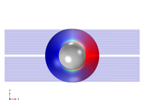
The wave vector, k (SI unit: 1/m) plays the same role in geometrical optics as the momentum, p, of particles in classical mechanics.
|
|
•
|


|
1
|
|
2
|
|
3
|
Click Add.
|
|
4
|
Click
|
|
5
|
|
6
|
Click
|
|
1
|
|
2
|
|
1
|
|
2
|
|
3
|
|
4
|
|
5
|
|
6
|
|
1
|
|
2
|
|
3
|
|
1
|
|
2
|
|
3
|
|
4
|
|
5
|
|
1
|
|
2
|
|
3
|
|
4
|
Browse to the model’s Application Libraries folder and double-click the file ideal_cloak_variables.txt.
|
|
1
|
|
2
|
In the Settings window for Mathematical Particle Tracing, locate the Particle Release and Propagation section.
|
|
3
|
|
1
|
In the Model Builder window, under Component 1 (comp1)>Mathematical Particle Tracing (pt) click Particle Properties 1.
|
|
2
|
|
3
|
|
4
|
|
1
|
|
2
|
|
3
|
|
4
|
|
5
|
|
1
|
|
2
|
|
3
|
|
5
|
Click to expand the Element Size Parameters section. Locate the Element Size section. Click the Custom button.
|
|
6
|
|
7
|
In the associated text field, type hmax_cloak.
|
|
8
|
|
9
|
In the associated text field, type hmax_cloak/2.
|
|
1
|
|
2
|
|
3
|
Click the Custom button.
|
|
4
|
|
5
|
|
6
|
|
1
|
|
2
|
|
3
|
Click
|
|
4
|
|
5
|
|
6
|
|
7
|
Click Replace.
|
|
8
|
|
9
|
|
10
|
|
1
|
|
2
|
|
3
|
|
4
|
|
5
|
|
6
|
|
7
|
|
8
|
|
9
|
|
1
|
|
2
|
|
3
|
|
4
|
|
1
|
In the Model Builder window, expand the Results>Particle Trajectories (pt)>Particle Trajectories 1 node, then click Particle Trajectories 1.
|
|
2
|
|
3
|
|
4
|
|
1
|
|
2
|
|
3
|
|
1
|
|
2
|
|
3
|
|
4
|
|
5
|
|
6
|
|
1
|
|
1
|
|
2
|
|
3
|
|
4
|
|
5
|
|
1
|
|
1
|
|
2
|
|
3
|
|
1
|
In the Model Builder window, under Results>Particle Trajectories (pt) click Particle Trajectories 1.
|
|
2
|
|
1
|
|
2
|
|
3
|
|
4
|
|
5
|
|
1
|
|
2
|
|
3
|
|
1
|
|
2
|
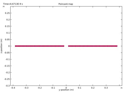
In the Settings window for 2D Plot Group, type Ray Position Relative to Initial Position in the Label text field.
|
|
3
|
|
4
|
In the associated text field, type y-position (m).
|
|
5
|
|
6
|
In the associated text field, type z-position (m).
|
|
1
|
|
2
|
|
3
|
|
4
|
|
5
|
|
1
|
|
2
|
|
3
|
|
4
|
|
5
|
|
7
|
|
8
|
|
1
|
|
2
|
|
3
|
|
4
|
|
5
|
|
6
|
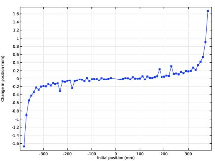
In the associated text field, type Initial position (mm).
|
|
7
|
|
8
|
In the associated text field, type Change in position (mm).
|
|
1
|
|
2
|
|
3
|
|
4
|
|
5
|
|
6
|
|
7
|
|
8
|
|
9
|
Click to expand the Coloring and Style section. Find the Line markers subsection. From the Marker list, choose Point.
|
|
10
|
|
11
|