
|
|
|
|
•
|
|
•
|
|
•
|
|
•
|
|
•
|
|
•
|
The turbulent kinetic energy k (SI unit: m2/s2) represents the energy per unit mass associated with eddies in the flow.
|
|
•
|
The turbulent dissipation rate ε (SI unit: m2/s3) indicates the rate at which turbulent kinetic energy in the eddies is converted to thermal energy.
|
|
•
|
The ratio k/ε has units of time. The average eddy lifetime is often estimated by multiplying this ratio by a dimensionless constant of order unity.
|
|
•
|
The ratio k3/2/ε has units of length and indicates the length scale of the largest eddies in the flow.
|

|
•
|
|
•
|
q (SI unit: m) is the particle position, and
|
|
•
|
|
•
|
|
•
|
|
•
|
CD (dimensionless) is the drag coefficient.
|

|
•
|
The Discrete Random Walk (DRW) model is similar to the modified Eddy Interaction Model of Gosman and Ioannides (Ref. 3). In the DRW model, unique velocity perturbations are sampled and added to the mean velocity field at discrete times based on the estimated eddy lifetime.
|
|
•
|
The Continuous Random Walk (CRW) model, or Continuous Filter White Noise (CFWN) model (Ref. 4). In the CRW model, the velocity perturbations are integrated over time. The eddy velocity and lifetime are built into the time derivatives of the evolving velocity perturbation components.
|


|
1
|
|
2
|
In the Select Physics tree, select Fluid Flow>Single-Phase Flow>Turbulent Flow>Turbulent Flow, k-ε (spf).
|
|
3
|
Click Add.
|
|
4
|
Click
|
|
5
|
|
6
|
Click
|
|
1
|
|
2
|
|
3
|
|
4
|
Browse to the model’s Application Libraries folder and double-click the file flow_channel_turbulent_dispersion_parameters.txt.
|
|
1
|
|
2
|
|
3
|
|
4
|
|
5
|
|
1
|
|
2
|
|
3
|
|
4
|
Click
|
|
5
|
|
1
|
In the Model Builder window, under Component 1 (comp1) right-click Materials and choose Blank Material.
|
|
2
|
|
1
|
In the Model Builder window, under Component 1 (comp1) right-click Turbulent Flow, k-ε (spf) and choose Inlet.
|
|
2
|
|
3
|
|
5
|
|
1
|
|
1
|
|
1
|
|
3
|
|
4
|
|
1
|
|
3
|
|
4
|
|
5
|
|
6
|
|
7
|
|
1
|
|
3
|
|
4
|
|
5
|
|
1
|
|
2
|
|
1
|
|
2
|
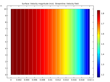
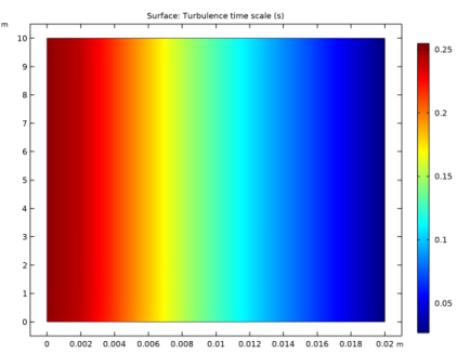
In the Settings window for Surface, click Replace Expression in the upper-right corner of the Expression section. From the menu, choose Component 1 (comp1)>Turbulent Flow, k-ε>Turbulence variables>spf.tauT - Turbulence time scale - s.
|
|
3
|
|
1
|
|
2
|
|
3
|
|
4
|
At the bottom of the Add Physics section, clear the check box next to Study 1. The particle trajectories are not solved for in the Stationary study step.
|
|
5
|
|
6
|
|
1
|
|
2
|
|
3
|
At the bottom of the Add Study section, clear the check box next to the Turbulent Flow, k-ε interface, which will not be solved for in the Time Dependent study step.
|
|
4
|
|
5
|
|
6
|
|
1
|
In the Model Builder window, under Component 1 (comp1)>Particle Tracing for Fluid Flow (fpt) click Particle Properties 1.
|
|
2
|
|
3
|
|
4
|
|
1
|
|
1
|
|
1
|
|
2
|
|
3
|
|
1
|
|
3
|
|
4
|
|
5
|
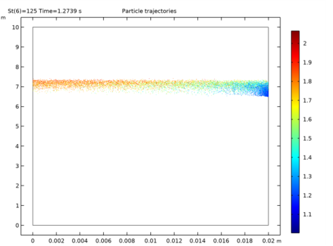
Locate the Turbulent Dispersion section. From the Turbulent dispersion model list, choose Continuous random walk.
|
|
6
|
|
7
|
|
8
|
|
9
|
|
1
|
|
2
|
|
3
|
|
4
|
|
5
|
|
6
|
|
7
|
|
8
|
Click Replace.
|
|
9
|
|
10
|
|
11
|
|
1
|
|
2
|
|
3
|
Click
|
|
1
|
|
2
|
|
3
|
|
4
|
Click to expand the Values of Dependent Variables section. Find the Values of variables not solved for subsection. From the Settings list, choose User controlled.
|
|
5
|
|
6
|
|
7
|
|
1
|
|
2
|
|
3
|
|
4
|
|
5
|
|
6
|
|
7
|
|
8
|
|
9
|
|
10
|
|
11
|
|
12
|
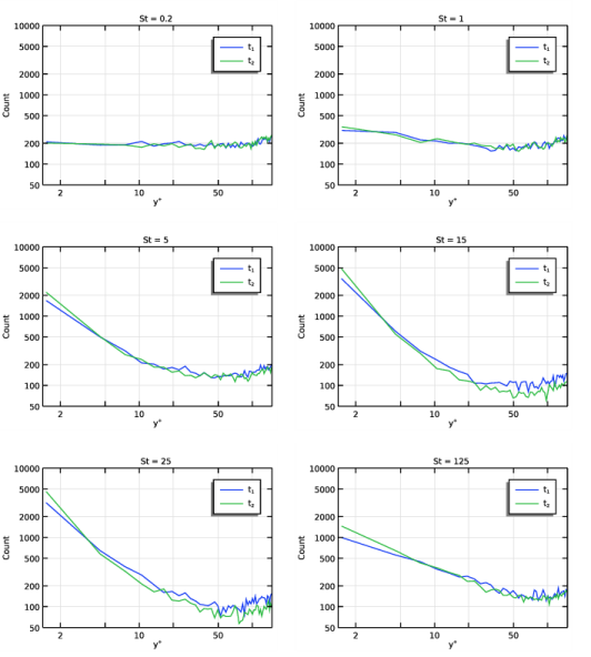
In the associated text field, type y<sup>+</sup>.
|
|
1
|
|
2
|
|
3
|
|
4
|
|
5
|
|
6
|
|
8
|
|
1
|
|
2
|
|
3
|
|
4
|
|
5
|
|
6
|
|
7
|
|
8
|
|
9
|
|
10
|