You are viewing the documentation for an older COMSOL version. The latest version is available here.
PDF

Parameter Optimization of a Tesla Microvalve
Introduction
A Tesla valve inhibits backward flow on a fixed geometry by utilizing friction forces instead of moving parts, Ref. 1. This means fluid can flow freely in one direction but not in the reverse direction. Typically the Reynolds number of the flow in microfluidics is between 1 and 100. This model sets up a parameter optimization model with inspiration from the model Optimization of a Tesla Microvalve, which finds a design for a Tesla valve using topology optimization. This model takes uncertainties in the form of erosion and dilation of the geometry into account using a parametric sweep and optimizes for the worst of three possible geometries.
Model Definition
The physics of this model is identical to that of Optimization of a Tesla Microvalve, so the main difference is in the setup of the parameterized geometry. The result of the topology optimization is shown in Figure 1, while the parameterized geometry for this model is shown in Figure 2.
Figure 1: The topology optimized design computed in the model, Optimization of a Tesla Microvalve.
Figure 2: The parameterized geometry used for this model is simple to allow for the use of a derivative free solver. Only half of the geometry is modeled, because this saves computational time.
The model is parameterized such that the topology of the geometry is fixed, while still allowing for the use of box constraints for the parameters. The erosion and dilation is implemented via the error parameter, which is used to scale the circles and the triangle. This parameter is then varied in a parametric sweep such that three different geometries are generated for every optimization iteration. Only the worst performing design is used to drive the optimization, but the worst design changes between the eroded and dilated design, so it is impossible to solve the problem using an outer sweep.
Results and Discussion
The result of the optimization is shown in Figure 3. As expected, it is not possible to achieve the same performance as for the topology optimized design, because the number of design variables goes from thousands to three. Therefore, the diodicity drops from 2.34 to 2.20 for the blue print design and 2.1 for the eroded/dilated designs.
Figure 3: The forward and backward flow is shown in the same plot for the blue print design. The eroded and dilated geometries are shown with black and white lines, respectively.
Reference
1. S. Lin, “Topology Optimization of Micro Tesla Valve in low and moderate Reynolds number,” Chinese Academy of Sciences, China, September 27, 2011 http://senlin.weebly.com/uploads/6/6/1/4/6614199/sen_lin_topology_optimization_of_micro_tesla_valve.pdf.
Notes About the COMSOL Implementation
The model is set up using two Laminar Flow interfaces, one for the forward flow and one for the reverse.
Application Library path: Optimization_Module/Design_Optimization/tesla_microvalve_parameter_optimization
Modeling Instructions
From the File menu, choose New.
New
In the New window, click  Model Wizard.
Model Wizard
1
In the Model Wizard window, click  2D.
2
In the Select Physics tree, select Fluid Flow>Single-Phase Flow>Laminar Flow (spf).
3
Click Add.
4
Click Add.
5
Click  Study.
6
In the Select Study tree, select General Studies>Stationary.
7
Geometry 1
Create the geometry. To simplify this step, insert a prepared geometry sequence.
1
In the Geometry toolbar, click  Insert Sequence.
2
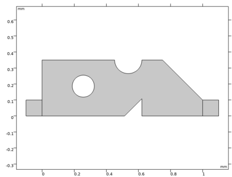
Browse to the model’s Application Libraries folder and double-click the file tesla_microvalve_parameter_optimization_geom_sequence.mph.
3
In the Geometry toolbar, click  Build All.
4
Click the  Zoom Extents button in the Graphics toolbar.
The geometry should now look like that in Figure 1. Note that the inserted geometry is parameterized and that the parameters used are automatically added to the list of global parameters in the model.
5
In the Model Builder window, collapse the Geometry 1 node.
Global Definitions
Geometrical Parameters
Add a new parameter group for calculating the average inlet velocity as a function of the Reynolds number.
1
In the Model Builder window, under Global Definitions click Parameters 1.
2
In the Settings window for Parameters, type Geometrical Parameters in the Label text field.
Parameters 2
1
In the Home toolbar, click  Parameters and choose Add>Parameters.
2
In the Settings window for Parameters, locate the Parameters section.
3
Definitions
Add the same nonlocal couplings and variables as for the topology optimization.
Average 1 (aveop1)
1
In the Definitions toolbar, click  Nonlocal Couplings and choose Average.
2
In the Settings window for Average, locate the Source Selection section.
3
From the Geometric entity level list, choose Boundary.
4
From the Selection list, choose Left.
Average 2 (aveop2)
1
In the Definitions toolbar, click  Nonlocal Couplings and choose Average.
2
In the Settings window for Average, locate the Source Selection section.
3
From the Geometric entity level list, choose Boundary.
4
From the Selection list, choose Right.
Integration 1 (intop1)
1
In the Definitions toolbar, click  Nonlocal Couplings and choose Integration.
2
Variables 1
1
In the Model Builder window, right-click Definitions and choose Variables.
2
In the Settings window for Variables, locate the Variables section.
3
Materials
Material 1 (mat1)
1
In the Model Builder window, under Component 1 (comp1) right-click Materials and choose Blank Material.
2
In the Settings window for Material, locate the Material Contents section.
3
Laminar Flow (spf)
Set up the same boundary conditions as for the topology optimization model.
Wall 2
1
In the Model Builder window, under Component 1 (comp1) right-click Laminar Flow (spf) and choose Wall.
2
In the Settings window for Wall, locate the Boundary Selection section.
3
From the Selection list, choose Symmetry.
4
Locate the Boundary Condition section. From the Wall condition list, choose Slip.
Inlet 1
1
In the Physics toolbar, click  Boundaries and choose Inlet.
2
In the Settings window for Inlet, locate the Boundary Selection section.
3
From the Selection list, choose Left.
4
Locate the Boundary Condition section. From the list, choose Fully developed flow.
5
Locate the Fully Developed Flow section. In the Uav text field, type Uin.
Outlet 1
1
In the Physics toolbar, click  Boundaries and choose Outlet.
2
In the Settings window for Outlet, locate the Boundary Selection section.
3
From the Selection list, choose Right.
Laminar Flow 2 (spf2)
In the Model Builder window, under Component 1 (comp1) click Laminar Flow 2 (spf2).
Wall 2
1
In the Physics toolbar, click  Boundaries and choose Wall.
2
In the Settings window for Wall, locate the Boundary Selection section.
3
From the Selection list, choose Symmetry.
4
Locate the Boundary Condition section. From the Wall condition list, choose Slip.
Inlet 1
1
In the Physics toolbar, click  Boundaries and choose Inlet.
2
In the Settings window for Inlet, locate the Boundary Selection section.
3
From the Selection list, choose Right.
4
Locate the Boundary Condition section. From the list, choose Fully developed flow.
5
Locate the Fully Developed Flow section. In the Uav text field, type Uin.
Outlet 1
1
In the Physics toolbar, click  Boundaries and choose Outlet.
2
In the Settings window for Outlet, locate the Boundary Selection section.
3
From the Selection list, choose Left.
Mesh 1
Generate an isotropic mesh with a minimum length scale of meshsz.
Free Triangular 1
In the Mesh toolbar, click  Free Triangular.
Size
1
In the Model Builder window, click Size.
2
In the Settings window for Size, locate the Element Size section.
3
From the Predefined list, choose Extremely fine.
4
Click the Custom button.
5
Locate the Element Size Parameters section. In the Maximum element size text field, type meshsz.
6
Click  Build All.
Initial design
Compute the flow and diodicity (Di) for the initial design.
1
In the Model Builder window, right-click Study 1 and choose Rename.
2
In the Rename Study dialog box, type Initial design in the New label text field.
3
4
In the Home toolbar, click  Compute.
Results
Global Evaluation 1
1
In the Results toolbar, click  Global Evaluation.
2
In the Settings window for Global Evaluation, locate the Expressions section.
3
Pressure (spf), Pressure (spf2), Velocity (spf), Velocity (spf2)
1
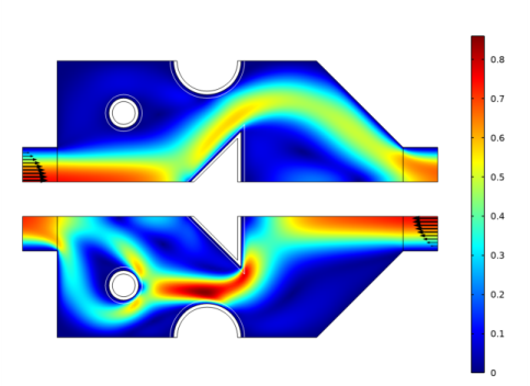
In the Model Builder window, under Results, Ctrl-click to select Velocity (spf), Pressure (spf), Velocity (spf2), and Pressure (spf2).
2
Initial Design
In the Settings window for Group, type Initial Design in the Label text field.
Root
Add a second study for the parameter optimization.
Add Study
1
In the Home toolbar, click  Add Study to open the Add Study window.
2
Go to the Add Study window.
3
Find the Studies subsection. In the Select Study tree, select General Studies>Stationary.
4
Click Add Study in the window toolbar.
5
In the Home toolbar, click  Add Study to close the Add Study window.
Study 2
Optimization
1
In the Study toolbar, click  Optimization.
2
In the Settings window for Optimization, locate the Optimization Solver section.
3
From the Method list, choose BOBYQA.
Use continuation in the Reynolds number to improve stability.
4
Click Add Expression in the upper-right corner of the Objective Function section. From the menu, choose Component 1 (comp1)>Definitions>Variables>comp1.Di - Ratio of pressure differences.
5
Locate the Objective Function section. From the Type list, choose Maximization.
6
Locate the Control Variables and Parameters section. Click  Addthree times.
7
Step 1: Stationary
1
In the Model Builder window, click Step 1: Stationary.
2
In the Settings window for Stationary, click to expand the Study Extensions section.
3
Select the Auxiliary sweep check box.
4
5
Add a Parametric sweep to take under- and overetching into account.
Parametric Sweep
1
In the Study toolbar, click  Parametric Sweep.
2
In the Settings window for Parametric Sweep, locate the Study Settings section.
3
4
Generate default plots to use while solving and use the worst solution to drive the optimization.
5
In the Model Builder window, click Study 2.
6
In the Settings window for Study, type Optimization in the Label text field.
7
In the Study toolbar, click  Get Initial Value.
Optimization
1
In the Model Builder window, click Optimization.
2
In the Settings window for Optimization, locate the Objective Function section.
3
From the Solution list, choose Use last.
4
From the Outer solution list, choose Minimum of objectives.
5
Locate the Output While Solving section. Select the Plot check box.
6
From the Plot group list, choose Velocity (spf2) 1.
7
In the Study toolbar, click  Compute.
Results
Pressure (spf) 1, Pressure (spf2) 1, Velocity (spf) 1, Velocity (spf2) 1
1
In the Model Builder window, under Results, Ctrl-click to select Velocity (spf) 1, Pressure (spf) 1, Velocity (spf2) 1, and Pressure (spf2) 1.
2
Optimized
In the Settings window for Group, type Optimized in the Label text field.
Evaluate the diodicity again.
Global Evaluation 1
1
In the Model Builder window, click Global Evaluation 1.
2
In the Settings window for Global Evaluation, locate the Data section.
3
From the Dataset list, choose Optimization/Parametric Solutions 1 (sol3).
4
Click  Evaluate.