You are viewing the documentation for an older COMSOL version. The latest version is available here.
PDF

Exporting and Importing a
Topology-Optimized Hook
Introduction
Topology optimization in a structural mechanics context can answer the question: Given that you know the loads on the structure, which distribution of the available material maximizes stiffness? Or, conversely, how much material is necessary to obtain a predefined stiffness, and how should it be distributed? Such investigations typically occur during the concept design stages.
The conflicting goals of stiffness maximization and mass minimization lead to a continuum of possible optimal solutions, depending on how you balance the goals against each other. This topology optimization example demonstrates how to use a penalization method (SIMP) to obtain an optimal distribution of a fixed amount of material such that stiffness is maximized. Changing the amount of material available leads to a different solution, which is also Pareto optimal, representing a different balance between the conflicting objectives.
Model Definition
The model studies optimal material distribution in a hook, which is symmetric about the plane z = 0 and consists of a linear elastic material, structural steel. It is subjected to two distributed load cases: One at the tip of the hook and one along its lower inner curve. The geometry is imported as a geometry sequence (Figure 1).
Figure 1: The computational domain of the hook is reduced by exploiting symmetry.
The optimality criterion is defined by the objective function, which is chosen to be the total strain energy in this example. Note that the strain energy exactly balances the work done by the applied load, so minimizing the strain energy minimizes the displacement induced at the points where loads are applied, effectively minimizing the compliance of the structure — maximizing its stiffness. The other, conflicting, objective is minimization of total mass, which is implemented as an upper bound on the mass of the optimized structure.
To regularize the problem we introduce a minimum length scale via a filter radius in a Helmholtz filter. See the Topology Optimization of an MBB Beam example for illustrations of this process. Ideally, the topology of the resulting designs should be mesh independent and for designs with moderate complexity this can be achieved, but if the optimal design is very complex, other designs with slightly different topologies perform only marginally worse, so the optimization problem has many local minima, and it is likely that a slightly suboptimal design is identified. The result of the optimization is shown in Figure 2.
Figure 2: A multislice plot colored with the displacement magnitude shows the topology optimized design before it is exported.
This example demonstrates a strategy based on using MMA with a limited number of iterations. The filtered variable is solved on a finer mesh to get a smooth design for postprocessing. You can use this to export a STL file, but to transfer the geometry to a 2nd component for verification purposes, it is best to use a Filter dataset. This approach enables the recycling of selections from the other component, but the parameters for the geometry Import feature can still require some tweaking to get a valid mesh for computation of the displacements in the imported geometry.
Results
The following plot shows the displacement field for the optimized solution after the geometry has been transferred and re-meshed.
Figure 3: A plot of the displacement field for the optimized design after it has been imported as an STL file.
Notes About the COMSOL Implementation
The control variable field, Helmholtz filter and SIMP penalization are defined through the use of a topology optimization feature. A Solid Mechanics interface represents the structural properties of the beam, while an Optimization interface allows adding the objective and the constraints for the optimization problem. The elastic strain energy density is a predefined variable, solid.Ws, available to use as the objective function for the optimization problem.
Only half of the hook geometry must be modeled, because of the assumed symmetry, which is implemented as a Symmetry condition on the symmetry plane. Plots for postprocessing and inspection of the solution while solving are set up using a Mirror data set, to show the complete solution. The geometry is parameterized, making it easy to experiment with different hook sizes, but keep in mind that the mesh size is taken as the filter radius.
The optimization solver is selected and controlled from an Optimization study step. For topology optimization, either the MMA or the SNOPT solver can be used. They have different merits and weaknesses. MMA tends to be braver in the beginning, proceeding quickly toward an approximate optimum, while SNOPT is more cautious but also converges more efficiently close to the final solution thanks to its second-order approximation of the objective.
Finally, it is worth noting that the problem of finding a stiff design can be quite different from finding a design that does not break and it is generally advised to use shape or parameter optimization to ensure that the design is free of excessive stress concentrations.
References
1. B.S. Lazarov and O. Sigmund, “Filters in topology optimization based on Helmholtz-type differential equations,” International Journal for Numerical Methods in Engineering, vol 86, pp. 765–781, 2011.
2. F. Wang, B.S. Lazarov and O. Sigmund, “On projection methods, convergence and robust formulations in topology optimization,” Structural and Multidisciplinary Optimization, vol 43, pp. 767–784, 2011.
3. M.P. Bendsøe, “Optimal shape design as a material distribution problem,” Structural Optimization, vol. 1, pp. 193–202, 1989.
Application Library path: Optimization_Module/Topology_Optimization/hook_optimization_stl
Modeling Instructions
From the File menu, choose New.
New
In the New window, click  Model Wizard.
Model Wizard
1
In the Model Wizard window, click  3D.
2
In the Select Physics tree, select Structural Mechanics>Solid Mechanics (solid).
3
Click Add.
4
Click  Study.
5
In the Select Study tree, select Preset Studies for Selected Physics Interfaces>Optimization>Topology Optimization, Stationary.
6
Geometry 1
Create the geometry. To simplify this step, insert a prepared geometry sequence.
1
In the Geometry toolbar, click  Insert Sequence.
2
3
In the Geometry toolbar, click  Build All.
4
Click the  Zoom Extents button in the Graphics toolbar.
The geometry should now look like that in Figure 1. Note that the inserted geometry is parameterized and that the parameters used are automatically added to the list of global parameters in the model.
Global Definitions
Geometric Parameters
1
In the Model Builder window, under Global Definitions click Parameters 1.
2
In the Settings window for Parameters, type Geometric Parameters in the Label text field.
Now there is a group for geometric parameters. Add a second group for parameters related to the optimization.
Parameters 2
1
In the Home toolbar, click  Parameters and choose Add>Parameters.
2
In the Settings window for Parameters, locate the Parameters section.
3
Mesh 1
Swept 1
1
In the Mesh toolbar, click  Swept.
2
In the Settings window for Swept, click to expand the Sweep Method section.
3
From the Face meshing method list, choose Triangular (generate prisms).
Size
1
In the Model Builder window, click Size.
2
In the Settings window for Size, locate the Element Size section.
3
Click the Custom button.
4
Locate the Element Size Parameters section. In the Maximum element size text field, type meshsz.
5
In the Minimum element size text field, type meshsz/4.
6
Click  Build All.
Use structural steel for the solid material.
Add Material
1
In the Home toolbar, click  Add Material to open the Add Material window.
2
Go to the Add Material window.
3
In the tree, select Built-in>Structural steel.
4
Click Add to Global Materials in the window toolbar.
5
In the Home toolbar, click  Add Material to close the Add Material window.
Materials
Topology Link 1 (toplnk1)
1
In the Settings window for Topology Link, locate the Link Settings section.
2
From the Material list, choose Structural steel (mat1).
The Young’s modulus is now coupled to the material. Next, set up a mirror dataset for seeing the full design, while optimizing.
Definitions
Density Model 1 (dtopo1)
1
In the Model Builder window, under Component 1 (comp1)>Definitions>Topology Optimization click Density Model 1 (dtopo1).
2
In the Settings window for Density Model, locate the Geometric Entity Selection section.
3
From the Selection list, choose Optimized Domains.
4
Locate the Filtering section. From the Rmin list, choose User defined.
5
6
Locate the Control Variable Discretization section. From the Element order list, choose Constant.
7
Locate the Control Variable Initial Value section. In the θ0 text field, type volfrac.
Prescribed Material 1
1
In the Definitions toolbar, click  Optimization and choose Prescribed Material.
2
In the Settings window for Prescribed Material, locate the Geometric Entity Selection section.
3
From the Selection list, choose Fixed Domain.
Add a Material Boundary Density and Void Boundary Density feature to avoid 90 degree angles at domain boundaries. In this case, these features will also cause the optimization to find design without internal cavities.
Prescribed Material Boundary 1
1
In the Definitions toolbar, click  Optimization and choose Prescribed Material Boundary.
2
In the Settings window for Prescribed Material Boundary, locate the Geometric Entity Selection section.
3
From the Selection list, choose Load Boundaries.
Prescribed Void Boundary 1
1
In the Definitions toolbar, click  Optimization and choose Prescribed Void Boundary.
2
In the Settings window for Prescribed Void Boundary, locate the Geometric Entity Selection section.
3
From the Selection list, choose Free Boundaries.
Variables 1
In the Model Builder window, right-click Definitions and choose Variables.
In topology optimization the geometry is not sufficiently well defined to warrant 2nd order shape functions.
Solid Mechanics (solid)
1
In the Settings window for Solid Mechanics, click to expand the Discretization section.
2
From the Displacement field list, choose Linear.
Fixed Constraint 1
1
Right-click Component 1 (comp1)>Solid Mechanics (solid) and choose Fixed Constraint.
2
In the Settings window for Fixed Constraint, locate the Boundary Selection section.
3
From the Selection list, choose Hole.
Symmetry 1
1
In the Physics toolbar, click  Boundaries and choose Symmetry.
2
In the Settings window for Symmetry, locate the Boundary Selection section.
3
From the Selection list, choose Symmetry.
Take both loads into account using the load case functionality.
Boundary Load 1
1
In the Physics toolbar, click  Boundaries and choose Boundary Load.
2
In the Settings window for Boundary Load, locate the Boundary Selection section.
3
From the Selection list, choose 1st Load Boundary.
4
Locate the Force section. From the Load type list, choose Total force.
5
Specify the Ftot vector as
6
In the Physics toolbar, click  Load Group and choose New Load Group.
Boundary Load 2
1
In the Model Builder window, right-click Boundary Load 1 and choose Duplicate.
2
In the Settings window for Boundary Load, locate the Boundary Selection section.
3
From the Selection list, choose 2nd Load Boundary.
4
In the Physics toolbar, click  Load Group and choose New Load Group.
Optimization
1
In the Model Builder window, click Study 1.
2
In the Settings window for Study, type Optimization in the Label text field.
Step 1: Stationary
1
In the Model Builder window, under Optimization click Step 1: Stationary.
2
In the Settings window for Stationary, click to expand the Study Extensions section.
3
Select the Define load cases check box.
4
5
6
Initialize the study to generate plots to show while solving.
7
In the Study toolbar, click  Get Initial Value.
Results
Mirror 3D 1
1
In the Results toolbar, click  More Datasets and choose Mirror 3D.
2
In the Settings window for Mirror 3D, locate the Data section.
3
From the Dataset list, choose Filter.
4
Locate the Plane Data section. From the Plane list, choose xy-planes.
Threshold
1
In the Model Builder window, expand the Results>Topology Optimization node, then click Threshold.
2
In the Settings window for 3D Plot Group, locate the Data section.
3
From the Dataset list, choose Mirror 3D 1.
Optimization
Topology Optimization
1
In the Model Builder window, under Optimization click Topology Optimization.
2
In the Settings window for Topology Optimization, locate the Optimization Solver section.
3
In the Maximum number of iterations text field, type 25.
The control variable will not converge to the tolerance in so few iterations, but the actual design will not change noticeably by using more iterations.
4
Locate the Constraints section. In the table, enter the following settings:
5
Locate the Output While Solving section. Select the Plot check box.
6
From the Plot group list, choose Threshold.
7
In the Home toolbar, click  Compute.
The optimization has removed material near the tip of the hook.
Results
Output material volume factor
1
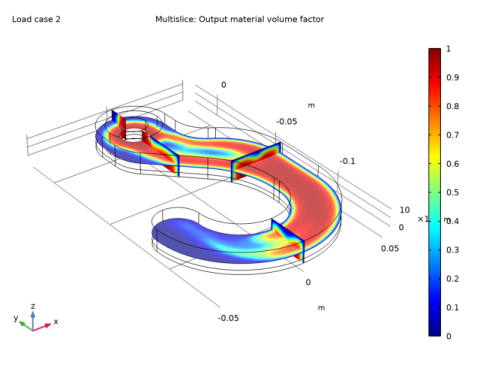
In the Model Builder window, under Results>Topology Optimization click Output material volume factor.
2
In the Output material volume factor toolbar, click  Plot.
3
Click the  Zoom Extents button in the Graphics toolbar.
Add a finer mesh and solve for the filtered material volume factor on this.
Mesh 1
In the Model Builder window, under Component 1 (comp1) right-click Mesh 1 and choose Duplicate.
Mesh 2
Size
1
In the Model Builder window, expand the Mesh 2 node, then click Size.
2
In the Settings window for Size, locate the Element Size Parameters section.
3
In the Maximum element size text field, type meshsz2.
4
In the Minimum element size text field, type meshsz2/4.
5
Click  Build All.
Add Study
1
In the Home toolbar, click  Add Study to open the Add Study window.
2
Go to the Add Study window.
3
Find the Studies subsection. In the Select Study tree, select General Studies>Stationary.
4
Find the Physics interfaces in study subsection. In the table, clear the Solve check box for Solid Mechanics (solid).
5
Click Add Study in the window toolbar.
6
In the Home toolbar, click  Add Study to close the Add Study window.
Smooth Design (mesh2)
1
In the Model Builder window, click Study 2.
2
In the Settings window for Study, type Smooth Design (mesh2) in the Label text field.
Solution 2 (sol2)
In the Study toolbar, click  Show Default Solver.
Step 1: Stationary
1
In the Model Builder window, expand the Solution 2 (sol2) node, then click Smooth Design (mesh2)>Step 1: Stationary.
2
In the Settings window for Stationary, click to expand the Values of Dependent Variables section.
3
Find the Initial values of variables solved for subsection. From the Settings list, choose User controlled.
4
From the Method list, choose Solution.
5
From the Study list, choose Optimization, Stationary.
6
In the Study toolbar, click  Compute.
Results
Filter 1
Create a new component from the filter dataset.
Add Component
In the Model Builder window, right-click the root node and choose Add Component>3D.
Mesh 3
Import 1
1
In the Mesh toolbar, click  Import.
2
In the Settings window for Import, locate the Import section.
3
From the Source list, choose Dataset.
4
From the Boundary partitioning list, choose Minimal.
5
Click Import.
Adapt 1
1
In the Mesh toolbar, click  Modify and choose Elements>Adapt.
2
In the Settings window for Adapt, locate the Adaptation section.
3
From the Solution list, choose None.
4
From the Type of expression list, choose Absolute size.
5
In the Size expression text field, type meshsz/2.
6
In the Maximum number of refinements text field, type 0.
7
In the Maximum coarsening factor text field, type Inf.
8
Click  Build Selected.
Free Tetrahedral 1
In the Mesh toolbar, click  Free Tetrahedral.
Size
1
In the Model Builder window, expand the Free Tetrahedral 1 node, then click Size.
2
In the Settings window for Size, locate the Element Size section.
3
From the Predefined list, choose Finer.
4
Click  Build All.
Use structural steel for the solid material.
Materials
Material Link 1 (matlnk1)
In the Model Builder window, under Component 2 (comp2) right-click Materials and choose More Materials>Material Link.
Solid Mechanics (solid)
Copy/paste the physics from the first component and fix the selections.
1
In the Model Builder window, under Component 1 (comp1) right-click Solid Mechanics (solid) and choose Copy.
Solid Mechanics (solid2)
1
In the Model Builder window, right-click Component 2 (comp2) and choose Paste Solid Mechanics.
2
In the Messages from Paste dialog box, click OK.
We can use 2nd order displacements now that we have an explicit geometry representation.
3
In the Model Builder window, click Solid Mechanics (solid2).
4
In the Settings window for Solid Mechanics, click to expand the Discretization section.
5
From the Displacement field list, choose Quadratic serendipity.
Fixed Constraint 1
1
In the Model Builder window, expand the Solid Mechanics (solid2) node, then click Fixed Constraint 1.
2
In the Settings window for Fixed Constraint, locate the Boundary Selection section.
3
From the Selection list, choose Hole.
Symmetry 1
1
In the Model Builder window, click Symmetry 1.
2
In the Settings window for Symmetry, locate the Boundary Selection section.
3
From the Selection list, choose Symmetry.
Boundary Load 1
1
In the Model Builder window, click Boundary Load 1.
2
In the Settings window for Boundary Load, locate the Boundary Selection section.
3
From the Selection list, choose 1st Load Boundary.
Boundary Load 2
1
In the Model Builder window, click Boundary Load 2.
2
In the Settings window for Boundary Load, locate the Boundary Selection section.
3
From the Selection list, choose 2nd Load Boundary.
Add Study
1
In the Home toolbar, click  Add Study to open the Add Study window.
2
Go to the Add Study window.
3
Find the Studies subsection. In the Select Study tree, select General Studies>Stationary.
4
Find the Physics interfaces in study subsection. In the table, clear the Solve check box for Solid Mechanics (solid).
5
Click Add Study in the window toolbar.
6
In the Model Builder window, click the root node.
7
In the Home toolbar, click  Add Study to close the Add Study window.
Optimization
Step 1: Stationary
1
In the Settings window for Stationary, locate the Physics and Variables Selection section.
2
In the table, clear the Solve for check box for Solid Mechanics (solid2).
Smooth Design (mesh2)
Step 1: Stationary
1
In the Model Builder window, under Smooth Design (mesh2) click Step 1: Stationary.
2
In the Settings window for Stationary, locate the Physics and Variables Selection section.
3
In the table, clear the Solve for check box for Solid Mechanics (solid2).
Study 3
Step 1: Stationary
1
In the Model Builder window, under Study 3 click Step 1: Stationary.
2
In the Settings window for Stationary, click to expand the Mesh Selection section.
3
4
Locate the Study Extensions section. Select the Define load cases check box.
5
6
7
8
In the Model Builder window, click Study 3.
9
In the Settings window for Study, type Verification in the Label text field.
10
Locate the Study Settings section. Clear the Generate default plots check box.
11
In the Home toolbar, click  Compute.
Add a new 3D plot group to plot the displacement.
Results
Displacement (solid2)
1
In the Home toolbar, click  Add Plot Group and choose 3D Plot Group.
2
In the Settings window for 3D Plot Group, type Displacement (solid2) in the Label text field.
3
Locate the Data section. From the Dataset list, choose Verification/Solution 3 (4) (sol3).
Volume 1
Right-click Displacement (solid2) and choose Volume.
Displacement (solid2)
1
Click the  Zoom Extents button in the Graphics toolbar.
2
In the Displacement (solid2) toolbar, click  Plot.
Topology Optimization 1
In the Model Builder window, right-click Topology Optimization 1 and choose Delete.