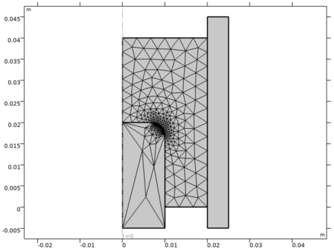
PDF

Powder Compaction of a Cup
Introduction
In this example, the fabrication of a cup through powder compaction is simulated. The powder compaction process is becoming common in the manufacturing industry, thanks to its potential to produce components of complex shape and high strength.
Combining the Fleck-Kuhn-McMeeking (FKM) model with the Gurson-Tvergaard-Needleman (GTN) model for porous plasticity makes it possible to cover a wide range of porosity values. Friction between the metal powder and the die is taken in to account. From a simulation point of view, this is a highly nonlinear structural analysis because of the contact interaction between the moving parts, the elastoplastic constitutive law selected for the metal powder, and the geometrical nonlinearity caused by the large displacements.
Model Definition
The geometry of workpiece (metal powder) and die are shown in Figure 1. The punch to compact the workpiece is not modeled. Instead, a prescribed displacement in the normal direction is used to compact the powder. Due to the axial symmetry, the size of model can be reduced.
Figure 1: Geometry of the workpiece (metal powder) and die.
Material Properties
For the aluminum metal powder, an elastoplastic material model with a constitutive relation given by a combination of the Fleck–Kuhn–McMeeking (FKM) model and the Gurson–Tvergaard–Needleman (GTN) is used. The parameters for the FKM-GTN model are given below.
The material of the die is irrelevant, since it is assumed to be rigid. Hence, the rigid domain material model is selected for the die.
Boundary Conditions
The applied boundary conditions are:
Results
Figure 2 shows the volumetric plastic strain at the end of compaction process. At the middle of the fillet, the volumetric plastic strain is at its minimum. At ends of the fillet, the volumetric plastic strain is high. The volumetric plastic strain at the corner points of the workpiece are about 12%, probably due to the friction.
Figure 2: The volumetric plastic strain at the end of compaction.
The compaction process reduces the porosity of the aluminum powder and increases its density. This process also results in an increase in the strength of the component. Considering the type of geometry and loading, non-uniform changes in porosity are expected. Contours of the current void volume fraction or porosity are shown in Figure 3. The metal powder in the thin lower portion of the workpiece is more compacted than the material in the middle or top portion. At the central region near to the fillet, the metal powder is less compacted due to material sliding on the rounded corner.
Figure 3: Current void volume fraction at the end of compaction.
The von Mises stress along with effective plastic strain in the workpiece at the end of compaction is shown in Figure 4
Figure 4: The von-Mises stress in the workpiece at the end of compaction.
Notes About the COMSOL Implementation
To improve the convergence and speed up the computations a customized mesh is used. The curved boundaries in a contact are well resolved using finer mesh, while the straight edges of the rigid domains are meshed with single elements, see Figure 5. The mesh on rigid parts only serve to describe the geometry accurately.
The parametric steps in the solver settings are tuned according to the used mesh. Changes in the mesh size may cause slower convergence and could thus require a modified step size to obtain the solution efficiently.
Figure 5: Customized mesh.
Application Library path: Nonlinear_Structural_Materials_Module/Porous_Plasticity/powder_compaction_of_a_cup
Modeling Instructions
From the File menu, choose New.
New
In the New window, click  Model Wizard.
Model Wizard
1
In the Model Wizard window, click  2D Axisymmetric.
2
In the Select Physics tree, select Structural Mechanics>Solid Mechanics (solid).
3
Click Add.
4
Click  Study.
5
In the Select Study tree, select General Studies>Stationary.
6
Global Definitions
Parameters 1
1
In the Model Builder window, under Global Definitions click Parameters 1.
2
In the Settings window for Parameters, locate the Parameters section.
3
Geometry 1
Rectangle 1 (r1)
1
In the Geometry toolbar, click  Rectangle.
2
In the Settings window for Rectangle, locate the Size and Shape section.
3
In the Width text field, type 20[mm].
4
In the Height text field, type 40[mm].
Rectangle 2 (r2)
1
In the Geometry toolbar, click  Rectangle.
2
In the Settings window for Rectangle, locate the Size and Shape section.
3
In the Width text field, type 10[mm].
4
In the Height text field, type 20[mm].
Difference 1 (dif1)
1
In the Geometry toolbar, click  Booleans and Partitions and choose Difference.
2
3
In the Settings window for Difference, locate the Difference section.
4
Find the Objects to subtract subsection. Select the  Activate Selection toggle button.
5
6
Click  Build Selected.
Fillet 1 (fil1)
1
In the Geometry toolbar, click  Fillet.
2
On the object dif1, select Point 4 only.
It might be easier to select the correct point by using the Selection List window. To open this window, in the Home toolbar click Windows and choose Selection List. (If you are running the cross-platform desktop, you find Windows in the main menu.)
3
In the Settings window for Fillet, locate the Radius section.
4
In the Radius text field, type 3[mm].
5
Click  Build Selected.
Rectangle 3 (r3)
1
In the Geometry toolbar, click  Rectangle.
2
In the Settings window for Rectangle, locate the Size and Shape section.
3
In the Width text field, type 10[mm].
4
In the Height text field, type 25[mm].
5
Locate the Position section. In the z text field, type -5[mm].
6
Click  Build Selected.
Fillet 2 (fil2)
1
In the Geometry toolbar, click  Fillet.
2
On the object r3, select Point 3 only.
3
In the Settings window for Fillet, locate the Radius section.
4
In the Radius text field, type 3[mm].
Rectangle 4 (r4)
1
In the Geometry toolbar, click  Rectangle.
2
In the Settings window for Rectangle, locate the Size and Shape section.
3
In the Width text field, type 5[mm].
4
In the Height text field, type 50[mm].
5
Locate the Position section. In the r text field, type 20[mm].
6
In the z text field, type -5[mm].
7
Click  Build All Objects.
Form Union (fin)
1
In the Model Builder window, under Component 1 (comp1)>Geometry 1 click Form Union (fin).
2
In the Settings window for Form Union/Assembly, locate the Form Union/Assembly section.
3
From the Action list, choose Form an assembly.
4
From the Pair type list, choose Contact pair.
5
In the Geometry toolbar, click  Build All.
6
Click  Build Selected.
Definitions
Add a Rigid Domain material model for domains 1 and 3 (die), and fix the domains. Set the density to zero as it does not affect the analysis.
Solid Mechanics (solid)
Rigid Domain 1
1
In the Model Builder window, expand the Component 1 (comp1)>Definitions node.
2
Right-click Component 1 (comp1)>Solid Mechanics (solid) and choose Material Models>Rigid Domain.
3
4
In the Settings window for Rigid Domain, locate the Density section.
5
From the ρ list, choose User defined.
Fixed Constraint 1
In the Physics toolbar, click  Attributes and choose Fixed Constraint.
For the elastoplastic analysis of the workpiece, choose the FKM-GTN porous plasticity model by adding a Porous Plasticity subnode to the Linear Elastic Material.
Linear Elastic Material 1
In the Model Builder window, click Linear Elastic Material 1.
Porous Plasticity 1
1
In the Physics toolbar, click  Attributes and choose Porous Plasticity.
2
In the Settings window for Porous Plasticity, locate the Porous Plasticity Model section.
3
From the Yield function F list, choose FKM-GTN.
Assign aluminum material properties to domain 2 (workpiece).
Materials
Aluminum
1
In the Model Builder window, under Component 1 (comp1) right-click Materials and choose Blank Material.
2
In the Settings window for Material, type Aluminum in the Label text field.
3
4
Locate the Material Contents section. In the table, enter the following settings:
Solid Mechanics (solid)
Contact 1
1
In the Physics toolbar, click  Pairs and choose Contact.
2
In the Settings window for Contact, locate the Pair Selection section.
3
Under Pairs, click  Add.
4
In the Add dialog box, in the Pairs list, choose Contact Pair 1 (ap1) and Contact Pair 2 (ap2).
5
Friction 1
1
In the Physics toolbar, click  Attributes and choose Friction.
2
In the Settings window for Friction, locate the Friction Parameters section.
3
In the μ text field, type 0.1.
Prescribed Displacement 1
1
In the Physics toolbar, click  Boundaries and choose Prescribed Displacement.
2
3
In the Settings window for Prescribed Displacement, locate the Prescribed Displacement section.
4
Select the Prescribed in z direction check box.
5
In the u0z text field, type -para.
Prescribed Displacement 2
1
In the Physics toolbar, click  Boundaries and choose Prescribed Displacement.
2
3
In the Settings window for Prescribed Displacement, locate the Prescribed Displacement section.
4
Select the Prescribed in z direction check box.
5
In the u0z text field, type para.
Now create the mesh. Start by defining a refined mesh in the contact region between the inner die and the workpiece, specifically at the fillet. Use a single mesh element on the straight edges of the inner and outer die.
Mesh 1
Mapped 1
1
In the Mesh toolbar, click  Mapped.
2
In the Settings window for Mapped, locate the Domain Selection section.
3
From the Geometric entity level list, choose Domain.
4
Distribution 1
1
Right-click Mapped 1 and choose Distribution.
2
3
In the Settings window for Distribution, locate the Distribution section.
4
In the Number of elements text field, type 1.
Free Triangular 1
In the Mesh toolbar, click  Free Triangular.
Distribution 1
1
Right-click Free Triangular 1 and choose Distribution.
2
In the Settings window for Distribution, locate the Boundary Selection section.
3
From the Selection list, choose All boundaries.
4
Click  Clear Selection.
5
Click  Paste Selection.
6
In the Paste Selection dialog box, type 12 in the Selection text field.
7
8
In the Settings window for Distribution, locate the Distribution section.
9
In the Number of elements text field, type 12.
Distribution 2
1
In the Model Builder window, right-click Free Triangular 1 and choose Distribution.
2
In the Settings window for Distribution, locate the Boundary Selection section.
3
Click  Paste Selection.
4
In the Paste Selection dialog box, type 5 in the Selection text field.
5
6
In the Settings window for Distribution, locate the Distribution section.
7
In the Number of elements text field, type 27.
Distribution 3
1
Right-click Free Triangular 1 and choose Distribution.
2
3
In the Settings window for Distribution, locate the Distribution section.
4
In the Number of elements text field, type 1.
Free Triangular 1
Right-click Free Triangular 1 and choose Build All.
Study 1
Step 1: Stationary
Set up an auxiliary continuation sweep for the para parameter.
1
In the Model Builder window, under Study 1 click Step 1: Stationary.
2
In the Settings window for Stationary, click to expand the Study Extensions section.
3
Select the Auxiliary sweep check box.
4
5
Solution 1 (sol1)
1
In the Study toolbar, click  Show Default Solver.
2
In the Model Builder window, expand the Solution 1 (sol1) node.
The step size is tuned in order to improve the convergence.
3
In the Model Builder window, expand the Study 1>Solver Configurations>Solution 1 (sol1)>Stationary Solver 1 node, then click Parametric 1.
4
In the Settings window for Parametric, click to expand the Continuation section.
5
Select the Tuning of step size check box.
6
In the Initial step size text field, type 2e-7.
7
In the Minimum step size text field, type 2e-7.
8
In the Maximum step size text field, type 2e-5.
9
In the Study toolbar, click  Compute.
Results
Volumetric Plastic Strain
In the Settings window for 2D Plot Group, type Volumetric Plastic Strain in the Label text field.
Surface 1
1
In the Model Builder window, expand the Volumetric Plastic Strain node, then click Surface 1.
2
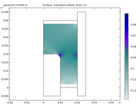
In the Settings window for Surface, click Replace Expression in the upper-right corner of the Expression section. From the menu, choose Component 1 (comp1)>Solid Mechanics>Strain>Strain invariants>solid.epvol - Volumetric plastic strain.
3
Locate the Coloring and Style section. From the Color table list, choose AuroraAustralisDark.
Volumetric Plastic Strain
1
In the Model Builder window, click Volumetric Plastic Strain.
2
In the Volumetric Plastic Strain toolbar, click  Plot.
In order to visualize the von Mises stress in the deformed workpiece along with undeformed dies, duplicate the Study 1/Solution 1 dataset, and set the selection to the domains 1 and 3. Set up a new Revolution 2D dataset based on Study 1/Solution 1 (2).
Study 1/Solution 1 (2) (sol1)
1
In the Model Builder window, expand the Results>Datasets node.
2
Right-click Results>Datasets>Study 1/Solution 1 (sol1) and choose Duplicate.
Selection
1
In the Results toolbar, click  Attributes and choose Selection.
2
In the Settings window for Selection, locate the Geometric Entity Selection section.
3
From the Geometric entity level list, choose Domain.
4
Revolution 2D 2
1
In the Model Builder window, under Results>Datasets right-click Revolution 2D 1 and choose Duplicate.
2
In the Settings window for Revolution 2D, locate the Data section.
3
From the Dataset list, choose Study 1/Solution 1 (2) (sol1).
von Mises Stress
1
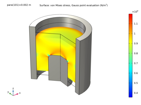
In the Model Builder window, expand the Results>Stress, 3D (solid) node, then click Stress, 3D (solid).
2
In the Settings window for 3D Plot Group, type von Mises Stress in the Label text field.
Surface 1
The Scale in Deformation node set to 2 in order to visualize the compaction.
Deformation
1
In the Model Builder window, expand the Results>von Mises Stress>Surface 1 node, then click Deformation.
2
In the Settings window for Deformation, locate the Scale section.
3
In the Scale factor text field, type 2.
von Mises Stress
In order to visualize undeformed dies, set up Surface 2 node by duplicating the Surface 1 node. Select the Revolution 2D 2 dataset, and type zero in the expression field. Add a Material Appearance node for the visualization.
Surface 2
1
In the Model Builder window, under Results>von Mises Stress right-click Surface 1 and choose Duplicate.
2
In the Settings window for Surface, locate the Data section.
3
From the Dataset list, choose Revolution 2D 2.
4
Locate the Expression section. In the Expression text field, type 0.
5
Click to expand the Title section. From the Title type list, choose None.
Material Appearance 1
1
Right-click Surface 2 and choose Material Appearance.
2
In the Settings window for Material Appearance, locate the Appearance section.
3
From the Appearance list, choose Custom.
4
From the Material type list, choose Steel.
5
In the von Mises Stress toolbar, click  Plot.
Current Void Volume Fraction (solid)
1
In the Model Builder window, click Current Void Volume Fraction (solid).
2
In the Current Void Volume Fraction (solid) toolbar, click  Plot.