|
|
|

|
•
|
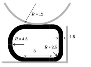
The rubber is hyperelastic and is modeled as a Mooney-Rivlin material with C10 = 0.37 MPa and C01 = 0.11 MPa. The material is almost incompressible, so the bulk modulus is set to 104 MPa. A mixed formulation is automatically used for this material model.
|
|
•
|
|
•
|
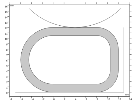
The rigid cylinder is lowered using the parameter of the parametric continuation solver as the negative y displacement. It starts with a gap of 0 mm and is lowered 4 mm.
|
|
1
|
|
2
|
|
3
|
Click Add.
|
|
4
|
Click
|
|
5
|
|
6
|
Click
|
|
1
|
|
2
|
|
3
|
|
1
|
|
2
|
|
3
|
|
4
|
|
5
|
|
6
|
|
7
|
Click to expand the Layers section. In the table, enter the following settings:
|
|
1
|
|
2
|
|
3
|
|
4
|
|
5
|
|
6
|
|
7
|
Locate the Layers section. In the table, enter the following settings:
|
|
1
|
|
2
|
|
3
|
|
4
|
|
5
|
|
6
|
|
7
|
|
8
|
Locate the Layers section. In the table, enter the following settings:
|
|
1
|
|
2
|
|
3
|
|
4
|
|
5
|
Click to expand the Layers section. In the table, enter the following settings:
|
|
1
|
|
2
|
|
3
|
|
4
|
|
5
|
|
6
|
|
7
|
|
8
|
|
1
|
|
2
|
|
3
|
|
4
|
On the object c1, select Domain 2 only.
|
|
5
|
On the object c2, select Domain 1 only.
|
|
6
|
On the object c3, select Domain 1 only.
|
|
7
|
On the object r1, select Domain 2 only.
|
|
1
|
|
2
|
Click in the Graphics window and then press Ctrl+A to select all objects.
|
|
3
|
|
4
|
|
1
|
|
2
|
|
3
|
|
4
|
|
5
|
|
6
|
|
7
|
|
8
|
Locate the Selections of Resulting Entities section. Select the Resulting objects selection check box.
|
|
9
|
|
1
|
|
2
|
|
3
|
|
4
|
|
5
|
|
6
|
Locate the Selections of Resulting Entities section. Select the Resulting objects selection check box.
|
|
7
|
|
8
|
|
9
|
|
10
|
Click OK.
|
|
1
|
|
2
|
|
3
|
|
4
|
|
5
|
Locate the Selections of Resulting Entities section. Find the Cumulative selection subsection. From the Contribute to list, choose Rigid base.
|
|
1
|
|
2
|
|
3
|
|
1
|
|
2
|
On the object ccur1, select Boundaries 1, 2, 4–6, and 8–10 only.
|
|
1
|
|
2
|
|
3
|
|
4
|
|
5
|
|
6
|
|
1
|
|
2
|
|
3
|
|
4
|
|
1
|
|
2
|
|
3
|
|
4
|
|
1
|
|
2
|
|
3
|
|
4
|
On the object fin, select Boundary 4 only.
|
|
1
|
|
2
|
|
1
|
|
2
|
|
3
|
|
4
|
|
1
|
|
2
|
|
3
|
|
4
|
|
1
|
|
2
|
|
3
|
|
4
|
|
5
|
|
1
|
|
2
|
|
3
|
|
1
|
|
2
|
|
3
|
|
4
|
Locate the Hyperelastic Material section. From the Material model list, choose Mooney-Rivlin, two parameters.
|
|
5
|
|
1
|
|
2
|
|
3
|
|
4
|
|
5
|
Click OK.
|
|
6
|
|
7
|
|
1
|
|
2
|
|
3
|
|
1
|
|
2
|
|
3
|
|
4
|
|
5
|
Click OK.
|
|
6
|
|
7
|
|
1
|
|
2
|
|
3
|
|
1
|
|
2
|
|
3
|
|
4
|
In the text field, type dom==4.
|
|
5
|
|
6
|
Specify the k vector as
|
|
1
|
|
2
|
|
3
|
|
4
|
|
1
|
|
2
|
|
1
|
|
2
|
|
3
|
|
4
|
|
5
|
|
1
|
In the Model Builder window, under Component 1 (comp1) right-click Materials and choose Blank Material.
|
|
2
|
|
1
|
|
1
|
|
2
|
|
3
|
|
4
|
|
1
|
|
2
|
|
3
|
|
4
|
|
1
|
|
2
|
|
3
|
|
4
|
|
5
|
|
6
|
|
8
|
|
1
|
|
2
|
|
3
|
|
4
|
In the Physics and variables selection tree, select Component 1 (comp1)>Solid Mechanics (solid), Controls spatial frame>Boundary Load 1.
|
|
5
|
Click
|
|
1
|
|
2
|
Click
|
|
4
|
|
5
|
|
6
|
|
1
|
In the Model Builder window, expand the Study: Without Pressure>Solver Configurations>Solution 1 (sol1) node.
|
|
2
|
In the Model Builder window, expand the Study: Without Pressure>Solver Configurations>Solution 1 (sol1)>Dependent Variables 1 node, then click Displacement field (comp1.u).
|
|
3
|
|
4
|
|
5
|
|
6
|
|
7
|
|
1
|
|
2
|
|
3
|
Select the Plot check box.
|
|
1
|
|
2
|
|
3
|
|
1
|
|
1
|
|
2
|
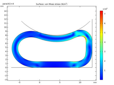
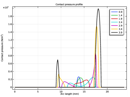
In the Settings window for 1D Plot Group, type Contact Pressure without Confined Air in the Label text field.
|
|
3
|
|
4
|
|
5
|
|
6
|
|
1
|
|
3
|
In the Settings window for Line Graph, click Replace Expression in the upper-right corner of the y-Axis Data section. From the menu, choose Component 1 (comp1)>Solid Mechanics>Contact>Contact 1>solid.cnt1.Tn - Contact pressure - N/m².
|
|
4
|
|
5
|
|
6
|
|
1
|
|
2
|
|
3
|
|
4
|
|
5
|
|
1
|
|
2
|
|
3
|
Click
|
|
5
|
|
6
|
|
7
|
|
8
|
|
9
|
|
10
|
Select the Plot check box.
|
|
11
|
|
1
|
In the Model Builder window, expand the Study: With Pressure>Solver Configurations>Solution 2 (sol2)>Dependent Variables 1 node, then click Displacement field (comp1.u).
|
|
2
|
|
3
|
|
4
|
|
5
|
|
6
|
|
1
|
|
2
|
|
3
|
|
4
|
|
5
|
|
1
|
In the Model Builder window, right-click Contact Pressure without Confined Air and choose Duplicate.
|
|
2
|
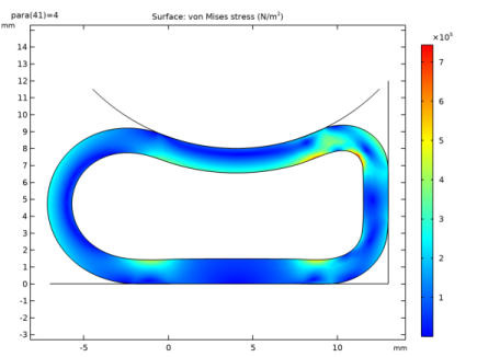
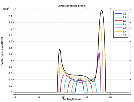
In the Settings window for 1D Plot Group, type Contact Pressure with Confined Air in the Label text field.
|
|
3
|
|
4
|
|
1
|
|
2
|
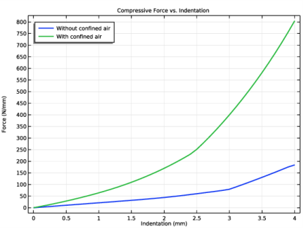
In the Settings window for 1D Plot Group, type Compressive Force vs. Indentation in the Label text field.
|
|
3
|
|
1
|
|
2
|
|
4
|
|
1
|
|
2
|
|
3
|
|
4
|
|
1
|
|
2
|
|
3
|
|
4
|
|
5
|
|
6
|
|
7
|