You are viewing the documentation for an older COMSOL version. The latest version is available here.
PDF

Twisting and Bending of a Metal Frame
Introduction
A thin-walled frame member with a central cutout is subjected to bending and twisting. The stresses around the cutout are expected to be above the yield stress of the material.
This example demonstrates how to model plastic deformation in thin structures. The Layered Linear Elastic Material in the Shell interface is used to define the load scenario, and the Plasticity subnode to quantify the plastic deformation around the cutout. The residual stress and plastic strains after removal of the load are investigated.
Model Definition
The load carrying beam is shown in Figure 1. It has a length of 1.1 m, a thin-walled square cross section with dimensions 160 x 160 mm2 and a wall thickness of 6 mm. The cutout is centrally placed on one of the faces and is 100 mm long, 80 mm wide, and has a fillet with a radius of 10 mm in each corner.
Figure 1: Geometry of the frame member.
The loading consists of a bending moments in the y direction, and a twisting moment around the x-axis. Both loads can vary independently and are applied at the right end of the frame at x = 1.1 m. The left end, x = 0, is clamped.
The frame is made out of steel with Young’s modulus, Poisson’s ratio, and density given as E = 200 GPa, ν = 0.33, and ρ = 7800 kg/m3, respectively. Yielding of the steel is governed by a von Mises plasticity model with an initial yield stress σys0 = 355 MPa. A tangent modulus Et = 100 MPa defines the isotropic hardening behavior.
Results and Discussion
Figure 2 shows the distribution of the von Mises stress at the peak of the applied loads. The effect of the cutout on the stress field is clearly visible. Due to the applied loads, stresses on the inner side of the frame are higher than on the outside.
Figure 2: Distribution of von Mises stress in the frame at the maximum load.
Figure 3 shows the residual stress on the outer surface of the frame after removal of the applied loads. Large stresses are visible in the vicinity of the cutout.
It is possible to observe the development of plastic strains in the structure during loading. Figure 4 shows the parts of the frame where plastic deformations have occurred at the end of the loading cycle. Note that plastic strains are not uniform through the shell thickness
Figure 3: Residual stress on the outside of the frame after removal of the applied loads
.
Figure 4: Equivalent plastic strain in the frame at end of the loading cycle.
Notes About the COMSOL Implementation
The structure is modeled with the Shell interface and the Layered Linear Elastic Material model. This feature enables to model phenomena that are thickness dependent, such as Plasticity. The user interface is similar to what is available in the Solid Mechanics interface.
In COMSOL Multiphysics, several load types can be applied to a Rigid Connector node. In this example, the Applied Moment node is used twice to apply a twisting moment around the x-axis, and a bending moment in the y direction. A piecewise function is used to ramp up the magnitude of these moments, and to remove the loads to observe the residual stress and plastic strains.
Application Library path: Nonlinear_Structural_Materials_Module/Plasticity/frame_with_cutout_plasticity
Modeling Instructions
From the File menu, choose New.
New
In the New window, click  Model Wizard.
Model Wizard
1
In the Model Wizard window, click  3D.
2
In the Select Physics tree, select Structural Mechanics>Shell (shell).
3
Click Add.
4
Click  Study.
5
In the Select Study tree, select General Studies>Stationary.
6
Global Definitions
Parameters 1
1
In the Model Builder window, under Global Definitions click Parameters 1.
2
In the Settings window for Parameters, locate the Parameters section.
3
Piecewise 1 (pw1)
1
In the Home toolbar, click  Functions and choose Global>Piecewise.
2
In the Settings window for Piecewise, locate the Definition section.
3
Find the Intervals subsection. In the table, enter the following settings:
4
Locate the Units section. In the Arguments text field, type 1.
5
In the Function text field, type N*m.
Geometry 1
Block 1 (blk1)
1
In the Geometry toolbar, click  Block.
2
In the Settings window for Block, locate the Object Type section.
3
From the Type list, choose Surface.
4
Locate the Size and Shape section. In the Width text field, type 1.1.
5
In the Depth text field, type 0.154.
6
In the Height text field, type 0.154.
7
Locate the Position section. From the Base list, choose Center.
Work Plane 1 (wp1)
1
In the Geometry toolbar, click  Work Plane.
2
In the Settings window for Work Plane, locate the Plane Definition section.
3
From the Plane type list, choose Face parallel.
4
On the object blk1, select Boundary 3 only.
5
Click  Show Work Plane.
Work Plane 1 (wp1)>Rectangle 1 (r1)
1
In the Work Plane toolbar, click  Rectangle.
2
In the Settings window for Rectangle, locate the Position section.
3
From the Base list, choose Center.
4
Locate the Size and Shape section. In the Width text field, type 80 [mm].
5
In the Height text field, type 100 [mm].
Work Plane 1 (wp1)>Fillet 1 (fil1)
1
In the Work Plane toolbar, click  Fillet.
2
On the object r1, select Points 1–4 only.
3
In the Settings window for Fillet, locate the Radius section.
4
In the Radius text field, type 10 [mm].
Difference 1 (dif1)
1
In the Model Builder window, right-click Geometry 1 and choose Booleans and Partitions>Difference.
2
3
In the Settings window for Difference, locate the Difference section.
4
Find the Objects to subtract subsection. Select the  Activate Selection toggle button.
5
Delete Entities 1 (del1)
1
Right-click Geometry 1 and choose Delete Entities.
2
On the object dif1, select Boundaries 1 and 6 only.
3
In the Settings window for Delete Entities, click  Build All Objects.
Add Material
1
In the Home toolbar, click  Add Material to open the Add Material window.
2
Go to the Add Material window.
3
In the tree, select Built-in>Structural steel.
4
Click  Add to Component 1 (comp1).
5
In the Home toolbar, click  Add Material to close the Add Material window.
Shell (shell)
Layered Linear Elastic Material 1
1
In the Model Builder window, under Component 1 (comp1) right-click Shell (shell) and choose Material Models>Layered Linear Elastic Material.
2
In the Settings window for Layered Linear Elastic Material, locate the Boundary Selection section.
3
From the Selection list, choose All boundaries.
Plasticity 1
In the Physics toolbar, click  Attributes and choose Plasticity.
Materials
Structural steel (mat1)
1
In the Model Builder window, under Component 1 (comp1)>Materials click Structural steel (mat1).
2
In the Settings window for Material, locate the Material Contents section.
3
Shell (shell)
Prescribed Displacement/Rotation 1
1
In the Physics toolbar, click  Edges and choose Prescribed Displacement/Rotation.
2
3
In the Settings window for Prescribed Displacement/Rotation, locate the Prescribed Displacement section.
4
Select the Prescribed in x direction check box.
5
Select the Prescribed in y direction check box.
6
Select the Prescribed in z direction check box.
Apply parametric twisting and bending moments at the other end using a rigid connector.
Rigid Connector 1
1
In the Physics toolbar, click  Edges and choose Rigid Connector.
2
Twisting Moment (x)
1
In the Physics toolbar, click  Attributes and choose Applied Moment.
2
In the Settings window for Applied Moment, type Twisting Moment (x) in the Label text field.
3
Locate the Applied Moment section. Specify the M vector as
Bending Moment (y)
1
Right-click Twisting Moment (x) and choose Duplicate.
2
In the Settings window for Applied Moment, type Bending Moment (y) in the Label text field.
3
Locate the Applied Moment section. Specify the M vector as
Create a custom mesh in order to increase the mesh density around the cutout.
Mesh 1
Free Triangular 1
In the Mesh toolbar, click  Boundary and choose Free Triangular.
Size
1
In the Model Builder window, click Size.
2
In the Settings window for Size, locate the Element Size section.
3
Click the Custom button.
4
Locate the Element Size Parameters section. In the Maximum element size text field, type 0.022.
5
In the Minimum element size text field, type 2.2E-4.
6
In the Maximum element growth rate text field, type 1.2.
7
In the Curvature factor text field, type 0.2.
8
In the Resolution of narrow regions text field, type 1.
Free Triangular 1
1
In the Model Builder window, click Free Triangular 1.
2
In the Settings window for Free Triangular, locate the Boundary Selection section.
3
From the Selection list, choose All boundaries.
Size Expression 1
1
Right-click Free Triangular 1 and choose Size Expression.
2
In the Settings window for Size Expression, locate the Element Size Expression section.
3
In the Size expression text field, type if((abs(X)>0.12)||(Y>0),0.022,0.008).
4
In the Number of cells per dimension text field, type 50.
5
Click  Build All.
Study 1
Step 1: Stationary
1
In the Model Builder window, under Study 1 click Step 1: Stationary.
2
In the Settings window for Stationary, click to expand the Study Extensions section.
3
Select the Auxiliary sweep check box.
4
5
6
In the Home toolbar, click  Compute.
Results
Stress (shell)
1
In the Settings window for 3D Plot Group, locate the Data section.
2
From the Dataset list, choose Layered Material 1.
3
From the Parameter value (para) list, choose 1.
4
Locate the Color Legend section. Select the Show maximum and minimum values check box.
Surface 1
1
In the Model Builder window, expand the Stress (shell) node, then click Surface 1.
2
In the Stress (shell) toolbar, click  Plot.
3
Click the  Zoom Extents button in the Graphics toolbar.
Stress, Slice (shell)
1
In the Model Builder window, click Stress, Slice (shell).
2
In the Settings window for 3D Plot Group, locate the Color Legend section.
3
Select the Show maximum and minimum values check box.
4
In the Model Builder window, expand the Stress, Slice (shell) node.
Deformation
1
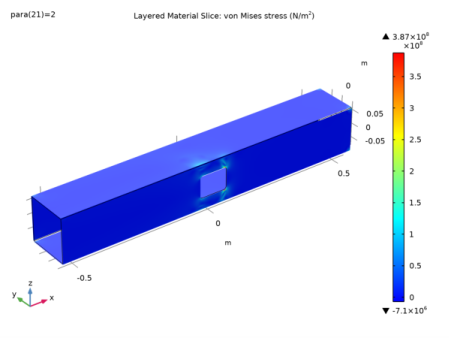
In the Model Builder window, expand the Results>Stress, Slice (shell)>Layered Material Slice 1 node, then click Deformation.
2
In the Settings window for Deformation, locate the Scale section.
3
Select the Scale factor check box.
4
5
In the Stress, Slice (shell) toolbar, click  Plot.
6
Click the  Zoom Extents button in the Graphics toolbar.
Contour 1
1
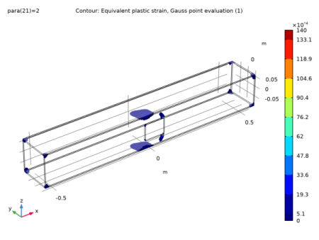
In the Model Builder window, expand the Equivalent Plastic Strain (shell) node, then click Contour 1.
2
In the Settings window for Contour, locate the Coloring and Style section.
3
From the Color table list, choose Rainbow.
Filter 1
1
Right-click Contour 1 and choose Filter.
2
In the Settings window for Filter, locate the Element Selection section.
3
In the Logical expression for inclusion text field, type shell.epeGp>1E-5.
4
In the Equivalent Plastic Strain (shell) toolbar, click  Plot.
Stress, Through Thickness (shell)
1
In the Model Builder window, click Stress, Through Thickness (shell).
2
In the Settings window for 1D Plot Group, locate the Data section.
3
From the Parameter selection (para) list, choose From list.
4
In the Parameter values (para) list, select 1.
5
In the Stress, Through Thickness (shell) toolbar, click  Plot.
Through Thickness 1
1
In the Model Builder window, expand the Stress, Through Thickness (shell) node, then click Through Thickness 1.
2
In the Settings window for Through Thickness, locate the Selection section.
3
Click  Clear Selection.
4
5
Locate the x-Axis Data section. From the Unit list, choose MPa.
6
In the Stress, Through Thickness (shell) toolbar, click  Plot.