You are viewing the documentation for an older COMSOL version. The latest version is available here.
PDF

Powder Compaction of a Rotational Flanged Component
Introduction
The powder compaction process is becoming common in the manufacturing industry, thanks to its potential to produce components of complex shape and high strength. The mechanical properties of the produced component depends on the final density, therefore the importance of uniform densification. Large variations in density can make a part weak, which affects the overall quality of the component. Finite element analysis with a properly chosen constitutive material model is a handy tool that can provide detailed information about densification, punch forces, friction phenomena, plastic deformation, and internal stresses, in order to better understand the process and to improve the quality of the manufacturing process.
The constitutive material models that are relevant for this type of simulations can broadly be classified in two types:
1
2
In this example studies the compaction of a rotational flanged component made of iron powder. As the porosity of the powder is large before compaction, a granular material model like the Capped Drucker-Prager (DPC) model is best suited as argued in Ref. 1 and Ref. 2. The elastic regime is represented by a linear elastic material, while a large plastic strain formulation together with a DPC yield function is used for the plastic regime. Additionally, friction between the powder and the die is taken into account. Simultaneous movement of the top and bottom punches is applied to avoid mesh distortion and other numerical problems. The simulation is performed using a 2D structured mesh with a linear displacement field as reported in Ref. 2.
The same example is studied in Ref. 1 with isotropic multiplicative hyperelastoplasticity, and in Ref. 2 with isotropic additive nonlinear elastoplasticity. In COMSOL Multiphysics, a linear elastoplastic material model is used in the geometric nonlinear regime with a multiplicative finite plastic strain formulation. The elastoplastic material model used in COMSOL Multiphysics is different from that used in Ref. 1 and Ref. 2, so the material parameters are chosen such as to get results in a similar range.
Before analyzing the rotational flanged component, isotropic compression and triaxial tests are carried out with the chosen material model and properties. The simulation results are then compared with experimental results given in Ref. 3. A good agreement is obtained between results for the isotropic compression test, and an acceptable agreement is obtained for the triaxial test. In this model, the isotropic and triaxial tests are not presented.
Model Definition
The geometry of the workpiece (metal powder) and the die is shown in Figure 1. The punch that compacts the workpiece is not modeled. Instead, a prescribed displacement in the normal direction is used to compact the powder. Due to the axial symmetry, the size of model can be reduced.
Figure 1: Geometry of the workpiece (metal powder) and the die.
Material Properties
For the iron metal powder, an elastoplastic material model with a constitutive relation given by a combination of the linear elastic material model and the Capped Drucker–Prager (DPC) model is used. The material parameters are listed below.
The material of the die is irrelevant, since it is assumed to be rigid. Therefore, it does no require any physics nor material properties.
Boundary Conditions
A prescribed displacement boundary condition for the upper and lower faces of the metal powder. The displacement in the z direction is controlled by an interpolation function.
Contact
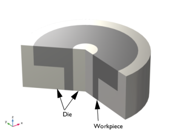
Since no physics is defined on the die, it is in the Contact node considered as external to the current physics.
The mesh on the source only needs to resolve the geometry of the contact surface. Hence no mesh is needed for the domain, but in order to show the die domains in the postprocessing plots the die domains are coarsely meshed.
Results and Discussion
As discussed in the introduction section of this documentation, the isotropic compression and triaxial tests are carried out with the same material model and properties. However, these tests are not part of the example, and only the results are presented for validation. A sample with an initial height of 24 mm and a diameter of 20 mm was used, see Ref. 1. The triaxial test is carried out by compacting the sample isotropically up to 50 MPa, and then axially compressing it while keeping the radial pressure constant at 50 MPa.
The simulation results are then compared with experimental results given in Ref. 3. Figure 2 shows that a good agreement is obtained between the simulation andthe experimental results for the isotropic compression test. Results from the triaxial test is presented in Figure 3 and Figure 4 that shows the variation of the current density and axial Cauchy stress with axial logarithmic strain. Both are in acceptable agreement with the experimental results from the triaxial test. The large difference in the evolution of the density in the triaxial test is due to a large difference at the initial isotropic stage, see Figure 2. Considering the fact that the elastoplastic material model used in COMSOL Multiphysics is different than that used in Ref. 1 and Ref. 2, differences in the results are expected. Nevertheless, the results show the same trend and are within an acceptable level. The results indicate that the chosen material model and properties can be used for analysis of the compaction of rotational flanged component, whose results are presented next.
.
Figure 2: Current density versus hydrostatic pressure in the isotropic compression test.
Figure 3: Current density versus axial logarithmic strain in the triaxial test.
Figure 4: Axial Cauchy stress versus axial logarithmic strain in the triaxial strain.
Figure 5 shows the volumetric plastic strain at the end of the compaction process. At the middle corner, the compressive volumetric plastic strain is at its minimum, while it at the top corner is at its maximum.
The compaction process reduces the porosity of the iron powder and increases its density. This process also results in an increase in the strength of the component. Considering the type of geometry and loading, nonuniform changes in porosity are expected. Contours of the current relative density in the middle and at the end of the compaction are shown in Figure 6 and Figure 7, respectively. The metal powder in the thin lower portion of the workpiece is more compacted than the material in the middle or top portion. At the corners, the metal powder is less compacted due to the friction effects, Ref. 2. Note that the relative densities presented in Ref. 1 and Ref. 2 do not match each other exactly due to the different elastoplastic material models and material properties, but they do show a similar trend. Along the same line, the results presented in the current example show the same trend as Ref. 1 and Ref. 2, and are also in close range with them.
Lastly, the von Mises stress along in the workpiece at the end of compaction is shown in Figure 8 in a 3D representation of the model.
Figure 5: Volumetric plastic strain at the end of compaction.
.
Figure 6: Current relative density in the middle of compaction.
Figure 7: Current relative density at the end of compaction.
Figure 8: Distribution of the von Mises stress in the workpiece at the end of the compaction process.
Notes About the COMSOL Implementation
The default contact method in COMSOL Multiphysics is the Penalty method, while the Augmented Lagrangian method is a more accurate but can also be more computationally expensive. The Augmented Lagrangian method comes in two flavors based on solution strategy: Fully Coupled and Segregated. Each flavor has its own advantages, see the COMSOL Multiphysics Reference Manual for further details.
The density distribution in the compaction process is affected by the contact pressure and the friction forces, so the accuracy of the contact algorithm is important in the powder compaction process. In this example, the Augmented Lagrangian method with a Fully Coupled solver is used. To get smooth convergence, parametric steps are adjusted and the Constant Newton method with a Linear predictor is used.
References
1. A. Perez-Foguet, A. Rodriguez-Ferran, and A. Huerta, “Consistent tangent matrices for density-dependent finite plasticity models,” Int. J. Numer. Anal. Meth. Geomech., vol. 25, pp. 1045–1075, 2001.
2. A.R. Khoei, A. Shamloo, and A.R. Azami, “Extended finite element method in plasticity forming of powder compaction with contact friction,” Int.J. Solids Struct., vol. 43, pp. 5421–5448, 2006.
3. P. Doremus, C.Geindreau, A. Martin, L.Debove, R. Lecot, and M. Dao, “High Pressure Triaxial Cell for Metal Powder”, Powder Metallurgy, vol. 38, no. 4, pp. 284–287, 1995.
Application Library path: Nonlinear_Structural_Materials_Module/Porous_Plasticity/compaction_of_a_rotational_flange
Modeling Instructions
From the File menu, choose New.
New
In the New window, click  Model Wizard.
Model Wizard
1
In the Model Wizard window, click  2D Axisymmetric.
2
In the Select Physics tree, select Structural Mechanics>Solid Mechanics (solid).
3
Click Add.
4
Click  Study.
5
In the Select Study tree, select General Studies>Stationary.
6
Global Definitions
Parameters 1
1
In the Model Builder window, under Global Definitions click Parameters 1.
2
In the Settings window for Parameters, locate the Parameters section.
3
Definitions
Before creating the geometry and setting up the physics, import the results of the isotropic compression test and the triaxial test done on an iron powder specimen with the same material properties and constitutive model as used in this example. Import also the experimental results of the isotropic compression test and the triaxial test done in Ref. 3.
Density in Isotropic Compression Test - Experiment
1
In the Model Builder window, expand the Component 1 (comp1)>Definitions node.
2
Right-click Definitions and choose Functions>Interpolation.
3
In the Settings window for Interpolation, type Density in Isotropic Compression Test - Experiment in the Label text field.
4
Locate the Definition section. Click  Load from File.
5
Browse to the model’s Application Libraries folder and double-click the file compaction_of_a_rotational_flange_isotropiccompression_experiment.txt.
Density in Isotropic Compression Test - Simulation
1
In the Home toolbar, click  Functions and choose Local>Interpolation.
2
In the Settings window for Interpolation, type Density in Isotropic Compression Test - Simulation in the Label text field.
3
Locate the Definition section. Click  Load from File.
4
Browse to the model’s Application Libraries folder and double-click the file compaction_of_a_rotational_flange_isotropiccompression_simulation.txt.
Density in Triaxial Test - Experiment
1
In the Home toolbar, click  Functions and choose Local>Interpolation.
2
In the Settings window for Interpolation, type Density in Triaxial Test - Experiment in the Label text field.
3
Locate the Definition section. Click  Load from File.
4
Browse to the model’s Application Libraries folder and double-click the file compaction_of_a_rotational_flange_triaxial_experiment1.txt.
Density in Triaxial Test - Simulation
1
In the Home toolbar, click  Functions and choose Local>Interpolation.
2
In the Settings window for Interpolation, type Density in Triaxial Test - Simulation in the Label text field.
3
Locate the Definition section. Click  Load from File.
4
Browse to the model’s Application Libraries folder and double-click the file compaction_of_a_rotational_flange_triaxial_simulation1.txt.
Axial Stress in Triaxial Test - Experiment
1
In the Home toolbar, click  Functions and choose Local>Interpolation.
2
In the Settings window for Interpolation, type Axial Stress in Triaxial Test - Experiment in the Label text field.
3
Locate the Definition section. Click  Load from File.
4
Browse to the model’s Application Libraries folder and double-click the file compaction_of_a_rotational_flange_triaxial_experiment2.txt.
Axial Stress in Triaxial Test - Simulation
1
In the Home toolbar, click  Functions and choose Local>Interpolation.
2
In the Settings window for Interpolation, type Axial Stress in Triaxial Test - Simulation in the Label text field.
3
Locate the Definition section. Click  Load from File.
4
Browse to the model’s Application Libraries folder and double-click the file compaction_of_a_rotational_flange_triaxial_simulation2.txt.
Create a plot from these interpolation functions in order to compare the experimental results with the results of the simulation.
Density in Isotropic Compression Test - Experiment (int1)
1
In the Model Builder window, under Component 1 (comp1)>Definitions click Density in Isotropic Compression Test - Experiment (int1).
2
In the Settings window for Interpolation, click  Create Plot.
Density in Isotropic Compression Test - Simulation (int2)
1
In the Model Builder window, under Component 1 (comp1)>Definitions click Density in Isotropic Compression Test - Simulation (int2).
2
In the Settings window for Interpolation, click  Create Plot.
Results
1D Plot Group 2
Combine the plots of the experimental and the simulation results of same type in one plot group, delete the unnecessary plots.
1
In the Model Builder window, under Results right-click 1D Plot Group 2 and choose Delete.
Density vs. Hydrostatic Pressure in Isotropic Compression Test
1
In the Model Builder window, under Results click 1D Plot Group 1.
2
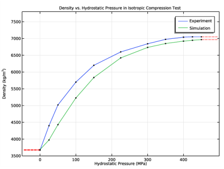
In the Settings window for 1D Plot Group, type Density vs. Hydrostatic Pressure in Isotropic Compression Test in the Label text field.
3
Click to expand the Title section. From the Title type list, choose Label.
4
Locate the Plot Settings section. Select the x-axis label check box.
5
In the associated text field, type Hydrostatic Pressure (MPa).
6
In the y-axis label text field, type Density (kg/m<sup>3</sup>).
7
Locate the Axis section. Select the Manual axis limits check box.
8
In the y minimum text field, type 3500.
9
In the y maximum text field, type 7800.
10
In the x maximum text field, type 500.
11
In the x minimum text field, type -50.
Function 1
1
In the Model Builder window, expand the Density vs. Hydrostatic Pressure in Isotropic Compression Test node, then click Function 1.
2
In the Settings window for Function, click to expand the Legends section.
3
Select the Show legends check box.
4
From the Legends list, choose Manual.
5
Function 2
1
Right-click Results>Density vs. Hydrostatic Pressure in Isotropic Compression Test>Function 1 and choose Duplicate.
2
In the Settings window for Function, locate the Data section.
3
From the Dataset list, choose Grid 1D 1a.
4
Locate the y-Axis Data section. In the Expression text field, type comp1.int2(t).
5
Locate the Output section. From the Point definition list, choose Cut Point 1D 2.
6
Locate the Legends section. In the table, enter the following settings:
7
In the Density vs. Hydrostatic Pressure in Isotropic Compression Test toolbar, click  Plot.
Definitions
Density in Triaxial Test - Experiment (int3)
1
In the Model Builder window, click Density in Triaxial Test - Experiment (int3).
2
In the Settings window for Interpolation, click  Create Plot.
Density in Triaxial Test - Simulation (int4)
1
In the Model Builder window, under Component 1 (comp1)>Definitions click Density in Triaxial Test - Simulation (int4).
2
In the Settings window for Interpolation, click  Create Plot.
Results
1D Plot Group 3
In the Model Builder window, under Results right-click 1D Plot Group 3 and choose Delete.
Density vs. Logarithmic Axial Strain in Triaxial Test
1
In the Model Builder window, under Results click 1D Plot Group 2.
2
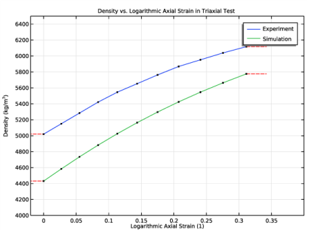
In the Settings window for 1D Plot Group, type Density vs. Logarithmic Axial Strain in Triaxial Test in the Label text field.
3
Locate the Title section. From the Title type list, choose Label.
4
Locate the Plot Settings section. Select the x-axis label check box.
5
In the associated text field, type Logarithmic Axial Strain (1).
6
In the y-axis label text field, type Density (kg/m<sup>3</sup>).
7
Locate the Axis section. Select the Manual axis limits check box.
8
In the y minimum text field, type 4000.
9
In the y maximum text field, type 6500.
10
In the x maximum text field, type 0.4.
11
In the x minimum text field, type -0.02.
Function 1
1
In the Model Builder window, expand the Density vs. Logarithmic Axial Strain in Triaxial Test node, then click Function 1.
2
In the Settings window for Function, locate the Legends section.
3
Select the Show legends check box.
4
From the Legends list, choose Manual.
5
Function 2
1
Right-click Results>Density vs. Logarithmic Axial Strain in Triaxial Test>Function 1 and choose Duplicate.
2
In the Settings window for Function, locate the Data section.
3
From the Dataset list, choose Grid 1D 1c.
4
Locate the y-Axis Data section. In the Expression text field, type comp1.int4(t).
5
Locate the Output section. From the Point definition list, choose Cut Point 1D 4.
6
Locate the Legends section. In the table, enter the following settings:
7
In the Density vs. Logarithmic Axial Strain in Triaxial Test toolbar, click  Plot.
Definitions
Axial Stress in Triaxial Test - Experiment (int5)
1
In the Model Builder window, click Axial Stress in Triaxial Test - Experiment (int5).
2
In the Settings window for Interpolation, click  Create Plot.
Axial Stress in Triaxial Test - Simulation (int6)
1
In the Model Builder window, under Component 1 (comp1)>Definitions click Axial Stress in Triaxial Test - Simulation (int6).
2
In the Settings window for Interpolation, click  Create Plot.
Results
1D Plot Group 4
In the Model Builder window, under Results right-click 1D Plot Group 4 and choose Delete.
Axial Cauchy Stress vs. Logarithmic Axial Strain in Triaxial Test
1
In the Model Builder window, under Results click 1D Plot Group 3.
2
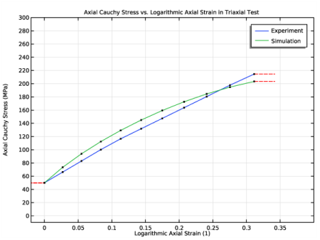
In the Settings window for 1D Plot Group, type Axial Cauchy Stress vs. Logarithmic Axial Strain in Triaxial Test in the Label text field.
3
Locate the Title section. From the Title type list, choose Label.
4
Locate the Plot Settings section. Select the x-axis label check box.
5
In the associated text field, type Logarithmic Axial Strain (1).
6
In the y-axis label text field, type Axial Cauchy Stress (MPa).
7
Locate the Axis section. Select the Manual axis limits check box.
8
In the y minimum text field, type -10.
9
In the y maximum text field, type 300.
10
In the x maximum text field, type 0.4.
11
In the x minimum text field, type -0.02.
Function 1
1
In the Model Builder window, expand the Axial Cauchy Stress vs. Logarithmic Axial Strain in Triaxial Test node, then click Function 1.
2
In the Settings window for Function, locate the Legends section.
3
Select the Show legends check box.
4
From the Legends list, choose Manual.
5
Function 2
1
Right-click Results>Axial Cauchy Stress vs. Logarithmic Axial Strain in Triaxial Test>Function 1 and choose Duplicate.
2
In the Settings window for Function, locate the Data section.
3
From the Dataset list, choose Grid 1D 1e.
4
Locate the y-Axis Data section. In the Expression text field, type comp1.int6(t).
5
Locate the Output section. From the Point definition list, choose Cut Point 1D 6.
6
Locate the Legends section. In the table, enter the following settings:
7
In the Axial Cauchy Stress vs. Logarithmic Axial Strain in Triaxial Test toolbar, click  Plot.
Now set up the model for compaction of a rotational flanged component.
Definitions
Top Punch Displacement
1
In the Home toolbar, click  Functions and choose Local>Interpolation.
2
In the Settings window for Interpolation, type Top Punch Displacement in the Label text field.
3
Locate the Definition section. In the Function name text field, type disp1.
4
5
Locate the Units section. In the Arguments text field, type s.
6
In the Function text field, type mm.
Bottom Punch Displacement
1
Right-click Top Punch Displacement and choose Duplicate.
2
In the Settings window for Interpolation, type Bottom Punch Displacement in the Label text field.
3
Locate the Definition section. In the Function name text field, type disp2.
4
Geometry 1
Rectangle 1 (r1)
1
In the Geometry toolbar, click  Rectangle.
2
In the Model Builder window, click Geometry 1.
3
In the Settings window for Geometry, locate the Units section.
4
From the Length unit list, choose mm.
5
In the Model Builder window, click Rectangle 1 (r1).
6
In the Settings window for Rectangle, locate the Size and Shape section.
7
In the Width text field, type 6.3.
8
In the Height text field, type 25.4.
9
Click  Build Selected.
Rectangle 2 (r2)
1
Right-click Rectangle 1 (r1) and choose Duplicate.
2
In the Settings window for Rectangle, locate the Size and Shape section.
3
In the Width text field, type 4.6.
4
In the Height text field, type 13.7.
5
Locate the Position section. In the r text field, type 6.3.
6
Click  Build Selected.
Rectangle 3 (r3)
1
Right-click Rectangle 2 (r2) and choose Duplicate.
2
In the Settings window for Rectangle, locate the Size and Shape section.
3
In the Width text field, type 20.2.
4
In the Height text field, type 11.7.
5
Locate the Position section. In the z text field, type 13.7.
6
Click  Build Selected.
Union 1 (uni1)
1
In the Geometry toolbar, click  Booleans and Partitions and choose Union.
2
Select the objects r2 and r3 only.
3
In the Settings window for Union, click  Build Selected.
Rectangle 4 (r4)
1
In the Model Builder window, under Component 1 (comp1)>Geometry 1 right-click Rectangle 3 (r3) and choose Duplicate.
2
In the Settings window for Rectangle, locate the Size and Shape section.
3
In the Width text field, type 15.6.
4
In the Height text field, type 13.7.
5
Locate the Position section. In the r text field, type 10.9.
6
In the z text field, type 0.
7
Click  Build Selected.
8
Click the  Zoom Extents button in the Graphics toolbar.
Rectangle 5 (r5)
1
Right-click Rectangle 4 (r4) and choose Duplicate.
2
In the Settings window for Rectangle, locate the Size and Shape section.
3
In the Width text field, type 6.3.
4
In the Height text field, type 25.4.
5
Locate the Position section. In the r text field, type 26.5.
6
Click  Build Selected.
Union 2 (uni2)
1
In the Geometry toolbar, click  Booleans and Partitions and choose Union.
2
Click the  Zoom Extents button in the Graphics toolbar.
3
Select the objects r4 and r5 only.
4
In the Settings window for Union, locate the Union section.
5
Clear the Keep interior boundaries check box.
6
Click  Build Selected.
Form Union (fin)
1
In the Model Builder window, under Component 1 (comp1)>Geometry 1 click Form Union (fin).
2
In the Settings window for Form Union/Assembly, locate the Form Union/Assembly section.
3
From the Action list, choose Form an assembly.
4
From the Pair type list, choose Contact pair.
5
Click  Build Selected.
Add the interior edge in the workpiece geometry to Mesh Control Edges in order to generate a structured mesh.
Mesh Control Edges 1 (mce1)
1
In the Geometry toolbar, click  Virtual Operations and choose Mesh Control Edges.
2
On the object fin, select Boundary 8 only.
3
In the Settings window for Mesh Control Edges, locate the Input section.
4
Clear the Include adjacent vertices check box.
5
Click  Build Selected.
In subsequent steps, the side domains will be not be part of the physics. Hence use the toggle button to switch the boundaries, so that the workpiece boundaries are chosen as destination boundaries.
Definitions
Contact Pair 2a (ap2)
1
In the Model Builder window, under Component 1 (comp1)>Definitions click Contact Pair 2a (ap2).
2
In the Settings window for Pair, click the  Swap Source and Destination button.
3
Locate the Source Boundaries section. Select the  Activate Selection toggle button.
4
Locate the Destination Boundaries section. Select the  Activate Selection toggle button.
Domains 1 and 3 (die) are considered as rigid and fixed, hence there is no need to consider them in physics, only a mesh is required.
Change the discretization to Linear.
Solid Mechanics (solid)
1
In the Model Builder window, under Component 1 (comp1) click Solid Mechanics (solid).
2
In the Settings window for Solid Mechanics, locate the Domain Selection section.
3
Click  Clear Selection.
4
5
Click to expand the Discretization section. From the Displacement field list, choose Linear.
For the elastoplastic analysis of the workpiece, choose Capped Drucker-Prager yield function with Large Plastic Strain porous plasticity model by adding a Porous Plasticity subnode to the Linear Elastic Material.
Linear Elastic Material 1
In the Model Builder window, under Component 1 (comp1)>Solid Mechanics (solid) click Linear Elastic Material 1.
Porous Plasticity 1
1
In the Physics toolbar, click  Attributes and choose Porous Plasticity.
2
In the Settings window for Porous Plasticity, locate the Porous Plasticity Model section.
3
From the Plasticity model list, choose Large plastic strains.
4
From the Yield function F list, choose Capped Drucker-Prager.
5
Find the Isotropic hardening model subsection. From the list, choose Exponential.
6
In the pb0 text field, type pc0.
For better accuracy, select the Augmented Lagrangian with a Fully Coupled solution method.
Contact 1
1
In the Physics toolbar, click  Pairs and choose Contact.
2
In the Settings window for Contact, locate the Pair Selection section.
3
Under Pairs, click  Add.
4
In the Add dialog box, in the Pairs list, choose Contact Pair 1a (ap1) and Contact Pair 2a (ap2).
5
6
In the Settings window for Contact, locate the Contact Surface section.
7
Select the Source external to current physics check box.
8
Locate the Contact Method section. From the Formulation list, choose Augmented Lagrangian.
9
From the Solution method list, choose Fully coupled.
Friction 1
1
In the Physics toolbar, click  Attributes and choose Friction.
2
In the Settings window for Friction, locate the Friction Parameters section.
3
In the μ text field, type mu.
Prescribed Displacement 1
1
In the Physics toolbar, click  Boundaries and choose Prescribed Displacement.
2
3
In the Settings window for Prescribed Displacement, locate the Prescribed Displacement section.
4
Select the Prescribed in z direction check box.
5
In the u0z text field, type disp1(t).
Prescribed Displacement 2
1
In the Physics toolbar, click  Boundaries and choose Prescribed Displacement.
2
3
In the Settings window for Prescribed Displacement, locate the Prescribed Displacement section.
4
Select the Prescribed in z direction check box.
5
In the u0z text field, type disp2(t).
Materials
Iron Powder
1
In the Model Builder window, under Component 1 (comp1) right-click Materials and choose Blank Material.
2
In the Settings window for Material, type Iron Powder in the Label text field.
3
4
Locate the Material Contents section. In the table, enter the following settings:
Mesh 1
Mapped 1
1
In the Mesh toolbar, click  Mapped.
2
In the Settings window for Mapped, locate the Domain Selection section.
3
From the Geometric entity level list, choose Domain.
4
5
Click to expand the Control Entities section. Clear the Smooth across removed control entities check box.
6
Click to expand the Reduce Element Skewness section. Select the Adjust edge mesh check box.
Distribution 1
1
Right-click Mapped 1 and choose Distribution.
2
3
In the Settings window for Distribution, locate the Distribution section.
4
In the Number of elements text field, type 4.
Distribution 2
1
In the Model Builder window, right-click Mapped 1 and choose Distribution.
2
3
In the Settings window for Distribution, locate the Distribution section.
4
In the Number of elements text field, type 20.
Mapped 2
1
In the Mesh toolbar, click  Mapped.
2
In the Settings window for Mapped, locate the Domain Selection section.
3
From the Geometric entity level list, choose Domain.
4
5
Click to expand the Control Entities section. Clear the Smooth across removed control entities check box.
6
Click to expand the Reduce Element Skewness section. Select the Adjust edge mesh check box.
Distribution 1
1
Right-click Mapped 2 and choose Distribution.
2
3
In the Settings window for Distribution, locate the Distribution section.
4
In the Number of elements text field, type 20.
Distribution 2
1
In the Model Builder window, right-click Mapped 2 and choose Distribution.
2
3
In the Settings window for Distribution, locate the Distribution section.
4
In the Number of elements text field, type 16.
Size
1
In the Model Builder window, click Size.
2
In the Settings window for Size, locate the Element Size section.
3
From the Predefined list, choose Coarser.
Free Quad 1
1
In the Mesh toolbar, click  Free Quad.
2
In the Settings window for Free Quad, click  Build All.
Augmented Lagrangian contact in addition to the material and geometric nonlinearity in the model demands special solver settings to achieve smooth convergence.
Study 1
Step 1: Stationary
Set up an auxiliary continuation sweep for the t parameter.
1
In the Model Builder window, under Study 1 click Step 1: Stationary.
2
In the Settings window for Stationary, click to expand the Study Extensions section.
3
Select the Auxiliary sweep check box.
4
5
Solution 1 (sol1)
1
In the Study toolbar, click  Show Default Solver.
2
In the Model Builder window, expand the Solution 1 (sol1) node.
Set up the solver in order to improve the convergence.
3
In the Model Builder window, expand the Study 1>Solver Configurations>Solution 1 (sol1)>Stationary Solver 1 node, then click Parametric 1.
4
In the Settings window for Parametric, click to expand the Continuation section.
5
Select the Tuning of step size check box.
6
In the Minimum step size text field, type 0.0005.
7
From the Predictor list, choose Linear.
8
In the Model Builder window, click Fully Coupled 1.
9
In the Settings window for Fully Coupled, click to expand the Method and Termination section.
10
From the Nonlinear method list, choose Constant (Newton).
11
From the Stabilization and acceleration list, choose Anderson acceleration.
12
In the Study toolbar, click  Compute.
Results
Study 1/Solution 1 (sol1)
In the Model Builder window, expand the Results>Datasets node, then click Study 1/Solution 1 (sol1).
Selection
1
In the Results toolbar, click  Attributes and choose Selection.
2
In the Settings window for Selection, locate the Geometric Entity Selection section.
3
From the Geometric entity level list, choose Domain.
4
Volumetric Plastic Strain
1
In the Model Builder window, under Results click Stress (solid).
2
In the Settings window for 2D Plot Group, type Volumetric Plastic Strain in the Label text field.
Surface 1
1
In the Model Builder window, expand the Volumetric Plastic Strain node, then click Surface 1.
2
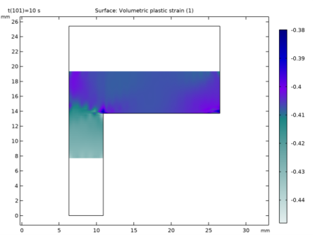
In the Settings window for Surface, click Replace Expression in the upper-right corner of the Expression section. From the menu, choose Component 1 (comp1)>Solid Mechanics>Strain>Strain invariants>solid.epvol - Volumetric plastic strain.
3
Locate the Coloring and Style section. From the Color table list, choose AuroraAustralisDark.
Volumetric Plastic Strain
1
In the Model Builder window, click Volumetric Plastic Strain.
2
In the Volumetric Plastic Strain toolbar, click  Plot.
In order to visualize the von Mises stress in the deformed workpiece along with the undeformed dies, duplicate the Study 1/Solution 1 dataset, and set the selection to domains 1 and 3. Set up a new Revolution 2D dataset based on Study 1/Solution 1 (2).
Study 1/Solution 1 (2) (sol1)
In the Model Builder window, under Results>Datasets right-click Study 1/Solution 1 (sol1) and choose Duplicate.
Selection
1
In the Model Builder window, expand the Study 1/Solution 1 (2) (sol1) node, then click Selection.
2
In the Settings window for Selection, locate the Geometric Entity Selection section.
3
Click  Clear Selection.
4
Revolution 2D 2
1
In the Model Builder window, under Results>Datasets right-click Revolution 2D 1 and choose Duplicate.
2
In the Settings window for Revolution 2D, locate the Data section.
3
From the Dataset list, choose Study 1/Solution 1 (2) (sol1).
In order to visualize the undeformed dies, set up Surface 2 node in the next 3D plot with a zero expression. Select the Revolution 2D 2 dataset, and add a Material Appearance node for the visualization..
von Mises Stress
1
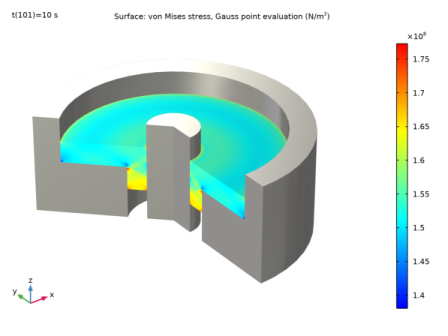
In the Model Builder window, expand the Results>Stress, 3D (solid) node, then click Stress, 3D (solid).
2
In the Settings window for 3D Plot Group, type von Mises Stress in the Label text field.
3
Locate the Plot Settings section. Clear the Plot dataset edges check box.
Surface 2
1
Right-click von Mises Stress and choose Surface.
2
In the Settings window for Surface, locate the Data section.
3
From the Dataset list, choose Revolution 2D 2.
4
Locate the Expression section. In the Expression text field, type 0.
5
Click to expand the Title section. From the Title type list, choose None.
Material Appearance 1
1
Right-click Surface 2 and choose Material Appearance.
2
In the Settings window for Material Appearance, locate the Appearance section.
3
From the Appearance list, choose Custom.
4
From the Material type list, choose Steel.
5
In the von Mises Stress toolbar, click  Plot.
Current Relative Density at Middle of Compaction
1
In the Model Builder window, under Results click Current Void Volume Fraction (solid).
2
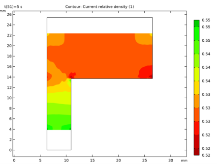
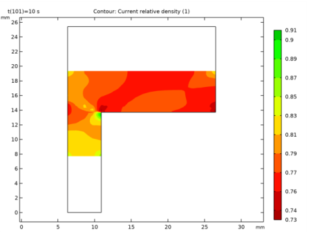
In the Settings window for 2D Plot Group, type Current Relative Density at Middle of Compaction in the Label text field.
3
Locate the Data section. From the Parameter value (t (s)) list, choose 5.
Contour 1
1
In the Model Builder window, expand the Current Relative Density at Middle of Compaction node, then click Contour 1.
2
In the Settings window for Contour, click Replace Expression in the upper-right corner of the Expression section. From the menu, choose Component 1 (comp1)>Solid Mechanics>Porous plasticity>solid.lemm1.popl1.rhorel - Current relative density.
3
Locate the Expression section. Clear the Description check box.
4
Locate the Coloring and Style section. Select the Reverse color table check box.
5
In the Current Relative Density at Middle of Compaction toolbar, click  Plot.
Current Relative Density at End of Compaction
1
In the Model Builder window, right-click Current Relative Density at Middle of Compaction and choose Duplicate.
2
In the Settings window for 2D Plot Group, type Current Relative Density at End of Compaction in the Label text field.
3
Locate the Data section. From the Parameter value (t (s)) list, choose 10.
4
In the Current Relative Density at End of Compaction toolbar, click  Plot.