Necking of an Elastoplastic Metal Bar

A circular bar of metal is subjected to a uniaxial tensile test. The the material presents an elastoplastic behavior with nonlinear isotropic hardening. When subjected to large deformations, the specimen experiences a significant plastic deformation and necking in its central cross section. This example demonstrates the large strain plasticity option available in the Nonlinear Structural Materials Module. The simulation results are compared with results in the literature.

Model Definition

In this model, a cylindrical steel bar with a height, H0, of 53.334 mm and a radius, R0, of 6.413 mm, is subjected to a total elongation of 14 mm.

The problem exhibits 2D axial symmetry as well as a reflection symmetry in the mid cross section of the bar. It is therefore possible to reduce the model geometry to a rectangle with a width equal to the radius of the bar, and a height equal to half of the length of the bar, see Figure 1.

The boundary conditions for the displacements in the radial and axial directions, u and w, that follow from the symmetries are

where r and z are the radial and axial coordinates. The tensile loadingis imposed through a prescribed elongation of Δ = 7 mm,

Figure 1: Schematic description of the numerical model. The red line shows the rotation symmetry axis.

Material Model

The elastic behavior of the material is characterized by a Young’s modulus E = 206.9 GPa and a Poisson’s ratio ν = 0.29. The plastic response follows a nonlinear isotropic hardening model with a yield stress given by

(1)

where σys0 is the initial yield stress and σh is the nonlinear hardening function. The latter is defined as

(2)

The hardening function σh depends nonlinearly on the equivalent plastic strain εpe. Here, H is the linear hardening coefficient, σysf is the saturation flow stress or residual yield stress, and ζ is the saturation exponent.

The numerical values of the parameters for the hardening function are given in Table 1. Figure 2, shows this nonlinear hardening as a function of equivalent plastic strain.

Table 1: Hardening function constants.
Constant	Value
σys0	450 MPa
H	129,24 MPa
σysf	715 MPa
ζ	16.93

Figure 2: Nonlinear isotropic hardening as a function of equivalent plastic strain.

Results and Discussion

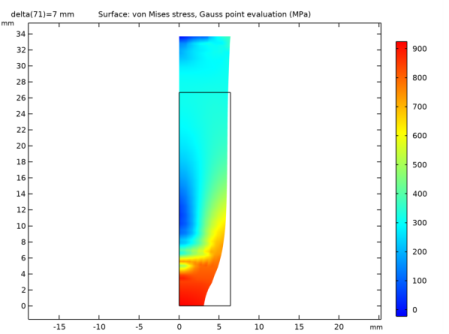
Figure 3 shows the distribution of the von Mises stress in the specimen. The figure also shows the deformation of the specimen, and how the nonlinear material behavior causes necking of its central cross section. The necking is caused by the very large plastic strains at the vertical symmetry plane as seen in Figure 4. A 7 mm elongation results in an equivalent plastic strain larger than 1.6 (this is, 160%) in the most affected region.

Figure 3: Distribution of the von Mises stress at 7 mm end displacement.

Figure 4: Distribution of the equivalent plastic strain at 7 mm end displacement. The results are shown in the undeformed configuration of the bar.

Figure 5 shows the change in radius as a function the elongation. Initially, the radius decreases linearly with the applied displacement. After an axial displacement of 3 mm, the radial reduction increases significantly and the specimen experiences necking. A similar case has been examined by Simo and Hughes (Ref. 1) as well as by Elguedj and Hughes (Ref. 2). Table 2 compares their results with the outcome of the current analysis. The calculated radial neck radius is in good agreement with results found in the literature.

Figure 5: Necking development in the mid section of the bar.

Table 2: Comparison between applied displacement and bar radius (mm) at the mid section.
δ (mm)	COMSOL	Ref. 1	Ref. 2
1.0	6.3	6.3	6.3
2.0	6.2	6.1	6.1
3.0	6.0	5.9	5.9
4.0	5.6	5.3	5.4
5.0	4.9	4.6	4.6
6.0	4.0	3.7	3.7

Notes About the COMSOL Implementation

The nonlinear hardening behavior is implemented using an analytic function. With reference to equation Equation 2, the hardening function is defined as

The user-defined hardening σh(εpe), portrayed in Figure 2, assumes zero stress for no plastic strain. In Equation 1, the yield stress is defined as the sum of the initial yield stress σys0 and the hardening function σh(εpe). The hardening function is defined in the node by an analytic function.

You find the option in the node. This option uses multiplicative decomposition between the elastic and plastic deformations, as opposed to additive decomposition which is used for the option. The small plastic strain assumption is generally not valid for strains above 0.1 (this is, more than 10%).

In this example, you use the double dogleg solver. This solver often works better for this class of nonlinear problems. The default Newton solver could also be used, but would then require tuning of the default solver settings.

References

1. J.C. Simo and T.R.J. Hughes, Computational Inelasticity, Springer, 2000.

2. T. Elguedj and T.J.R. Hughes, Isogeometric Analysis of Nearly Incompressible Large Strain Plasticity, ICES REPORT 11-35, the Institute for Computational Engineering and Sciences, the University of Texas at Austin, 2011.

Nonlinear_Structural_Materials_Module/Plasticity/bar_necking

Modeling Instructions

From the menu, choose .

New

In the window, click

Model Wizard

In the window, click

In the tree, select .

Click .

Click

In the tree, select .

Click

Global Definitions

Parameters 1

In the window, under click .

In the window for , locate the section.

In the table, enter the following settings:


Name	Expression	Value	Description
sigma0	450[MPa]	4.5E8 Pa	Initial yield stress
sigmaSF	715[MPa]	7.15E8 Pa	Saturation flow stress
H	129.24[MPa]	1.2924E8 Pa	Linear hardening coefficient
zeta	16.93	16.93	Saturation exponent
delta	0[m]	0 m	Top displacement
H0	53.334[mm]	0.053334 m	Bar length
R0	6.413[mm]	0.006413 m	Bar radius

Geometry 1

In the window, under click .

In the window for , locate the section.

From the list, choose .

Rectangle 1 (r1)

In the toolbar, click

In the window for , locate the section.

In the text field, type R0.

In the text field, type H0/2.

Click

Solid Mechanics (solid)

Prescribed Displacement, Bottom

In the window, under right-click and choose .

In the window for , type Prescribed Displacement, Bottom in the text field.

Select Boundary 2 only.

Locate the section. Select the check box.

Prescribed Displacement, Top

In the toolbar, click

and choose .

In the window for , type Prescribed Displacement, Top in the text field.

Select Boundary 3 only.

Locate the section. Select the check box.

Select the check box.

In the u 0 z text field, type delta.

Linear Elastic Material 1

In the window, click .

Plasticity 1

In the toolbar, click

and choose .

In the window for , locate the section.

From the list, choose .

Find the subsection. From the list, choose .

Materials

Material 1 (mat1)

In the window, under right-click and choose .

In the window for , locate the section.

In the table, enter the following settings:


Property	Variable	Value	Unit	Property group
Young’s modulus	E	206.9[GPa]	Pa	Basic
Poisson’s ratio	nu	0.29	1	Basic
Density	rho	7850	kg/m³	Basic
Initial yield stress	sigmags	sigma0	Pa	Elastoplastic material model