PDF

Inflation of a Spherical Rubber Balloon — Shell and Membrane Version
Introduction
The purpose of this example is to illustrate how the Shell and Membrane interfaces can be used to model deformation in thin hyperelastic structures. The model is identical to the Application Library example, Inflation of a Spherical Rubber Balloon, however, in this example, the Shell and Membrane interfaces are used instead of the Solid Mechanics interface.
When using the Membrane interface, the main difference is that it does not compute the variation across the thickness as the Solid Mechanics interface does, since the interface is based on the plane stress assumption for thin structures.
In contrast to the Membrane interface, the hyperelastic material in the Shell interface computes variations across the thickness direction by using the layered shell technology. Both the Membrane interface and the Shell interface share the same geometric dimension, but the Shell interface is a bit more computationally expensive compared to the Membrane interface due to the constitutive equation across the thickness and rotational degrees of freedom. However, since either the Membrane or the Shell interface are defined on a geometric dimension lower than a Solid Mechanics interface, the modeling with these interfaces is computationally more efficient.
All relevant details about the geometry and material parameters can be found in the Inflation of a Spherical Rubber Balloon example.
Results and Discussions
The results obtained with the Membrane and Shell interface are almost equivalent to the results from obtained in a Solid Mechanics interface.
Figure 1 shows the distribution of von Mises stress for a neo-Hookean material in the Shell interface at maximum inflation. The stress varies from 41.5 MPa to 42.2 MPa across the thickness, which agrees with the results obtained with the Solid Mechanics interface, where the stress varies from 41.4 MPa to 42.2 MPa across the thickness.
Figure 2 shows the distribution of von Mises stress for a neo-Hookean material in the Membrane interface at maximum inflation. A uniform stress though thickness of 41.83 MPa agrees well with the results obtained with the Solid Mechanics interface, where the stress varies from 41.4 MPa to 42.2 MPa across the thickness.
Figure 1: Distribution of von Mises stress for the neo-Hookean material in the shell interface at maximum inflation.
Figure 2: Distribution von Mises stress for the neo-Hookean material in the membrane interface at maximum inflation
The variation of inflation pressure versus applied stretch for different hyperelastic material models is shown in Figure 3. The inflation pressure in the Shell interface matches exactly the results shown in the Membrane interface. Also, the plot is identical to the results obtained with the Solid Mechanics interface for all material models.
Figure 3: Computed inflation pressure as a function of circumferential stretch for different material models, compared to the analytical expression for the Ogden material.
The variation of hoop stress versus applied stretch for different hyperelastic material models is shown in Figure 4. The hoop stress in the Shell interface matches exactly the results from the Membrane interface. The plot is identical to the results obtained with the Solid Mechanics interface for all material models.
Figure 5 shows a comparison of the trough thickness deformation in the Shell, Membrane and Solid Mechanics interfaces. The results from Shell, Membrane and Solid Mechanics versions match, so the thinning of the balloon can be accurately captured using either the Shell or Membrane interfaces, thus saving computational cost.
.
Figure 4: Computed hoop stress as a function of circumferential stretch for different material models, compared to the analytical expression for the Ogden material
.
Figure 5: Comparison of the trough thickness deformation in the Shell, Membrane and Solid Mechanics interfaces.
Notes About the COMSOL Implementation
The absence of bending stiffness in the Membrane interface requires a pre-stretching step before solving the inflation step. A separate study is created to compute this step, and the results from this study are used as initial values for the inflation step.
Although the Shell interface does not need a pre-stretching step, this step is computed anyways for easier comparison with the results from the Membrane interface.
Application Library path: Nonlinear_Structural_Materials_Module/Hyperelasticity/balloon_inflation_shell_membrane
Modeling Instructions
From the File menu, choose New.
New
In the New window, click  Model Wizard.
Model Wizard
1
In the Model Wizard window, click  2D Axisymmetric.
2
In the Select Physics tree, select Structural Mechanics>Shell (shell).
3
Click Add.
4
In the Select Physics tree, select Structural Mechanics>Membrane (mbrn).
5
Click Add.
6
Click  Study.
7
In the Select Study tree, select General Studies>Stationary.
8
Global Definitions
Begin by defining model parameters.
Parameters 1
1
In the Model Builder window, under Global Definitions click Parameters 1.
2
In the Settings window for Parameters, locate the Parameters section.
3
Setting the bulk modulus to 10^5 times the shear modulus is based on the assumption that the material is nearly incompressible.
Create an interpolation function of deformed thickens versus stretch. The imported data was computed with the Solid Mechanics interface.
Interpolation 1 (int1)
1
In the Home toolbar, click  Functions and choose Global>Interpolation.
2
In the Settings window for Interpolation, locate the Definition section.
3
Click  Load from File.
4
5
Locate the Units section. In the Arguments text field, type 1.
6
In the Function text field, type mm.
Definitions
Variables 1
1
In the Home toolbar, click  Variables and choose Local Variables.
2
In the Settings window for Variables, locate the Variables section.
3
Use the applied stretch and the inner radius of the balloon to compute the applied displacement.
Geometry 1
Due to symmetry, it suffices to model a 20-degree sector of the balloon.
Circle 1 (c1)
1
In the Geometry toolbar, click  Circle.
2
In the Settings window for Circle, locate the Object Type section.
3
From the Type list, choose Curve.
4
Locate the Size and Shape section. In the Radius text field, type Ri+H/2.
5
In the Sector angle text field, type 20.
Delete Entities 1 (del1)
1
In the Model Builder window, right-click Geometry 1 and choose Delete Entities.
2
On the object c1, select Boundaries 2 and 3 only.
3
In the Settings window for Delete Entities, click  Build Selected.
Add a Single Layer Material before adding a Layered Hyperelastic Material node in the shell interface.
Materials
Hyperelastic Material
1
In the Model Builder window, under Component 1 (comp1) right-click Materials and choose Layers>Single Layer Material.
2
In the Settings window for Material, type Hyperelastic Material in the Label text field.
3
Locate the Material Contents section. In the table, enter the following settings:
Shell (shell)
Neo-Hookean
1
In the Model Builder window, under Component 1 (comp1) right-click Shell (shell) and choose Material Models>Layered Hyperelastic Material.
2
In the Settings window for Layered Hyperelastic Material, type Neo-Hookean in the Label text field.
3
Locate the Boundary Selection section. From the Selection list, choose All boundaries.
4
Locate the Hyperelastic Material section. From the Compressibility list, choose Nearly incompressible material, quadratic volumetric strain energy.
5
From the μ list, choose User defined. In the associated text field, type mu.
6
In the κ text field, type kappa.
Mooney-Rivlin
1
In the Physics toolbar, click  Boundaries and choose Layered Hyperelastic Material.
2
In the Settings window for Layered Hyperelastic Material, type Mooney-Rivlin in the Label text field.
3
Locate the Boundary Selection section. From the Selection list, choose All boundaries.
4
Locate the Hyperelastic Material section. From the Material model list, choose Mooney-Rivlin, two parameters.
5
From the C10 list, choose User defined. In the associated text field, type 0.4375*mu.
6
From the C01 list, choose User defined. In the associated text field, type 0.0625*mu.
7
In the κ text field, type kappa.
Ogden
1
In the Physics toolbar, click  Boundaries and choose Layered Hyperelastic Material.
2
In the Settings window for Layered Hyperelastic Material, type Ogden in the Label text field.
3
Locate the Boundary Selection section. From the Selection list, choose All boundaries.
4
Locate the Hyperelastic Material section. From the Material model list, choose Ogden.
5
Click Add twice.
6
In the Ogden parameters table, enter the following settings:
7
In the κ text field, type kappa.
Varga
1
In the Physics toolbar, click  Boundaries and choose Layered Hyperelastic Material.
2
In the Settings window for Layered Hyperelastic Material, type Varga in the Label text field.
3
Locate the Boundary Selection section. From the Selection list, choose All boundaries.
4
Locate the Hyperelastic Material section. From the Material model list, choose Varga.
5
From the c1 list, choose User defined. In the associated text field, type 2*mu.
6
From the c2 list, choose User defined. In the κ text field, type kappa.
To enforce a symmetry constraint, use Prescribed Displacement nodes. Add a rotated coordinate system to enforce the symmetry constraint at the top.
Prescribed Displacement/Rotation 1
1
In the Physics toolbar, click  Points and choose Prescribed Displacement/Rotation.
2
3
In the Settings window for Prescribed Displacement/Rotation, locate the Prescribed Displacement section.
4
Select the Prescribed in z direction check box.
5
Locate the Prescribed Rotation section. From the By list, choose Rotation.
Definitions (comp1)
Rotated System 2 (sys2)
1
In the Definitions toolbar, click  Coordinate Systems and choose Rotated System.
2
In the Settings window for Rotated System, locate the Rotation section.
3
In the Rotation about out-of-plane axis text field, type 20[deg].
Shell (shell)
Prescribed Displacement/Rotation 2
1
In the Physics toolbar, click  Points and choose Prescribed Displacement/Rotation.
2
3
In the Settings window for Prescribed Displacement/Rotation, locate the Coordinate System Selection section.
4
From the Coordinate system list, choose Rotated System 2 (sys2).
5
Locate the Prescribed Displacement section. Select the Prescribed in x3 direction check box.
6
Locate the Prescribed Rotation section. From the By list, choose Rotation.
Prescribe the displacement in the normal direction for the prestretch analysis.
Prescribed Displacement/Rotation 3
1
In the Physics toolbar, click  Boundaries and choose Prescribed Displacement/Rotation.
2
In the Settings window for Prescribed Displacement/Rotation, locate the Boundary Selection section.
3
From the Selection list, choose All boundaries.
4
Locate the Coordinate System Selection section. From the Coordinate system list, choose Boundary System 1 (sys1).
5
Locate the Prescribed Displacement section. Select the Prescribed in n direction check box.
6
In the u0n text field, type -1[mm].
7
Locate the Prescribed Rotation section. From the By list, choose Rotation.
Control the inflation of the balloon by the pressure.
Face Load 1
1
In the Physics toolbar, click  Boundaries and choose Face Load.
2
In the Settings window for Face Load, locate the Boundary Selection section.
3
From the Selection list, choose All boundaries.
4
Locate the Force section. From the Load type list, choose Pressure.
5
In the p text field, type pf_s.
Define the pressure pf_s using a Global Equation feature. First, define a nonlocal integration coupling to evaluate the displacement at point 2.
Definitions (comp1)
Integration 1 (intop1)
1
In the Definitions toolbar, click  Nonlocal Couplings and choose Integration.
2
In the Settings window for Integration, locate the Source Selection section.
3
From the Geometric entity level list, choose Point.
4
5
Locate the Advanced section. From the Frame list, choose Material  (R, PHI, Z).
6
Clear the Compute integral in revolved geometry check box.
Variables 1
1
In the Model Builder window, click Variables 1.
2
In the Settings window for Variables, locate the Variables section.
3
4
Click the  Show More Options button in the Model Builder toolbar.
5
In the Show More Options dialog box, in the tree, select the check box for the node Physics>Equation-Based Contributions.
6
Click OK to enable a global equations and other advanced modeling features to the Shell and Membrane interfaces.
Shell (shell)
Global Equations 1
1
In the Physics toolbar, click  Global and choose Global Equations.
2
In the Settings window for Global Equations, locate the Global Equations section.
3
4
Locate the Units section. Click  Select Dependent Variable Quantity.
5
In the Physical Quantity dialog box, type pressure in the text field.
6
Click  Filter.
7
In the tree, select General>Pressure (Pa).
8
9
In the Settings window for Global Equations, locate the Units section.
10
Click  Select Source Term Quantity.
11
In the Physical Quantity dialog box, type length in the text field.
12
Click  Filter.
13
In the tree, select General>Length (m).
14
Membrane (mbrn)
Thickness and Offset 1
1
In the Model Builder window, under Component 1 (comp1)>Membrane (mbrn) click Thickness and Offset 1.
2
In the Settings window for Thickness and Offset, locate the Thickness and Offset section.
3
In the d text field, type H.
Add the four hyperelastic material models.
Neo-Hookean
1
In the Physics toolbar, click  Boundaries and choose Hyperelastic Material.
2
In the Settings window for Hyperelastic Material, type Neo-Hookean in the Label text field.
3
Locate the Boundary Selection section. From the Selection list, choose All boundaries.
4
Locate the Hyperelastic Material section. From the Compressibility list, choose Nearly incompressible material, quadratic volumetric strain energy.
5
From the μ list, choose User defined. In the associated text field, type mu.
6
In the κ text field, type kappa.
Mooney-Rivlin
1
In the Physics toolbar, click  Boundaries and choose Hyperelastic Material.
2
In the Settings window for Hyperelastic Material, type Mooney-Rivlin in the Label text field.
3
Locate the Boundary Selection section. From the Selection list, choose All boundaries.
4
Locate the Hyperelastic Material section. From the Material model list, choose Mooney-Rivlin, two parameters.
5
From the C10 list, choose User defined. In the associated text field, type 0.4375*mu.
6
From the C01 list, choose User defined. In the associated text field, type 0.0625*mu.
7
In the κ text field, type kappa.
Ogden
1
In the Physics toolbar, click  Boundaries and choose Hyperelastic Material.
2
In the Settings window for Hyperelastic Material, type Ogden in the Label text field.
3
Locate the Boundary Selection section. From the Selection list, choose All boundaries.
4
Locate the Hyperelastic Material section. From the Material model list, choose Ogden.
5
Click Add twice.
6
In the Ogden parameters table, enter the following settings:
7
In the κ text field, type kappa.
Varga
1
In the Physics toolbar, click  Boundaries and choose Hyperelastic Material.
2
In the Settings window for Hyperelastic Material, type Varga in the Label text field.
3
Locate the Boundary Selection section. From the Selection list, choose All boundaries.
4
Locate the Hyperelastic Material section. From the Material model list, choose Varga.
5
From the c1 list, choose User defined. In the associated text field, type 2*mu.
6
From the c2 list, choose User defined. In the κ text field, type kappa.
Prescribed Displacement 1
1
In the Physics toolbar, click  Points and choose Prescribed Displacement.
2
3
In the Settings window for Prescribed Displacement, locate the Prescribed Displacement section.
4
Select the Prescribed in z direction check box.
Prescribed Displacement 2
1
In the Physics toolbar, click  Points and choose Prescribed Displacement.
2
3
In the Settings window for Prescribed Displacement, locate the Coordinate System Selection section.
4
From the Coordinate system list, choose Rotated System 2 (sys2).
5
Locate the Prescribed Displacement section. Select the Prescribed in x3 direction check box.
Prescribed Displacement 3
1
In the Physics toolbar, click  Boundaries and choose Prescribed Displacement.
2
In the Settings window for Prescribed Displacement, locate the Boundary Selection section.
3
From the Selection list, choose All boundaries.
4
Locate the Coordinate System Selection section. From the Coordinate system list, choose Boundary System 1 (sys1).
5
Locate the Prescribed Displacement section. Select the Prescribed in n direction check box.
6
In the u0n text field, type -1[mm].
Control the inflation of the balloon by the pressure.
Face Load 1
1
In the Physics toolbar, click  Boundaries and choose Face Load.
2
In the Settings window for Face Load, locate the Boundary Selection section.
3
From the Selection list, choose All boundaries.
4
Locate the Force section. From the Load type list, choose Pressure.
5
In the p text field, type pf_m.
Define the pressure pf_m using a Global Equation feature.
Definitions (comp1)
Variables 1
1
In the Model Builder window, under Component 1 (comp1)>Definitions click Variables 1.
2
In the Settings window for Variables, locate the Variables section.
3
Membrane (mbrn)
Global Equations 1
1
In the Physics toolbar, click  Global and choose Global Equations.
2
In the Settings window for Global Equations, locate the Global Equations section.
3
4
Locate the Units section. Click  Select Dependent Variable Quantity.
5
In the Physical Quantity dialog box, type pressure in the text field.
6
Click  Filter.
7
In the tree, select General>Pressure (Pa).
8
9
In the Settings window for Global Equations, locate the Units section.
10
Click  Select Source Term Quantity.
11
In the Physical Quantity dialog box, type length in the text field.
12
Click  Filter.
13
In the tree, select General>Length (m).
14
Mesh 1
Edge 1
1
In the Mesh toolbar, click  Edge.
2
In the Settings window for Edge, locate the Boundary Selection section.
3
From the Selection list, choose All boundaries.
Distribution 1
1
Right-click Edge 1 and choose Distribution.
2
In the Settings window for Distribution, locate the Distribution section.
3
In the Number of elements text field, type 50.
4
Click  Build All.
Study: Prestretch
The first study solves for the prestretch analysis.
1
In the Model Builder window, click Study 1.
2
In the Settings window for Study, type Study: Prestretch in the Label text field.
3
Locate the Study Settings section. Clear the Generate default plots check box.
Step 1: Stationary
1
In the Model Builder window, under Study: Prestretch click Step 1: Stationary.
2
In the Settings window for Stationary, locate the Physics and Variables Selection section.
3
Select the Modify model configuration for study step check box.
4
In the Physics and variables selection tree, select Component 1 (comp1)>Shell (shell), Controls spatial frame.
5
Click  Control Frame Deformation.
6
In the Physics and variables selection tree, select Component 1 (comp1)>Shell (shell), Spatial frame control disabled>Face Load 1 and Component 1 (comp1)>Shell (shell), Spatial frame control disabled>Global Equations 1.
7
Click  Disable.
8
In the Physics and variables selection tree, select Component 1 (comp1)>Membrane (mbrn), Controls spatial frame>Face Load 1 and Component 1 (comp1)>Membrane (mbrn), Controls spatial frame>Global Equations 1.
9
Click  Disable.
Modify the default solver to improve convergence. Use manual scaling to help the nonlinear solver in the first steps.
Solution 1 (sol1)
1
In the Study toolbar, click  Show Default Solver.
2
In the Model Builder window, expand the Solution 1 (sol1) node.
3
In the Model Builder window, expand the Study: Prestretch>Solver Configurations>Solution 1 (sol1)>Dependent Variables 1 node, then click Displacement of shell normals (comp1.ar).
4
In the Settings window for Field, locate the Scaling section.
5
In the Scale text field, type 1e-9.
6
In the Study toolbar, click  Compute.
Add a study for the neo-Hookean material model, then repeat the steps described above.
Add Study
1
In the Study toolbar, click  Add Study to open the Add Study window.
2
Go to the Add Study window.
3
Find the Studies subsection. In the Select Study tree, select General Studies>Stationary.
4
Click Add Study in the window toolbar.
5
In the Study toolbar, click  Add Study to close the Add Study window.
Study: Neo-Hookean
1
In the Model Builder window, click Study 2.
2
In the Settings window for Study, type Study: Neo-Hookean in the Label text field.
3
Locate the Study Settings section. Clear the Generate default plots check box.
Step 1: Stationary
1
In the Model Builder window, under Study: Neo-Hookean click Step 1: Stationary.
2
In the Settings window for Stationary, locate the Physics and Variables Selection section.
3
Select the Modify model configuration for study step check box.
4
In the Physics and variables selection tree, select Component 1 (comp1)>Shell (shell), Controls spatial frame.
5
Click  Control Frame Deformation.
6
In the Physics and variables selection tree, select Component 1 (comp1)>Shell (shell), Spatial frame control disabled>Mooney-Rivlin, Component 1 (comp1)>Shell (shell), Spatial frame control disabled>Ogden, Component 1 (comp1)>Shell (shell), Spatial frame control disabled>Varga, and Component 1 (comp1)>Shell (shell), Spatial frame control disabled>Prescribed Displacement/Rotation 3.
7
Click  Disable.
8
In the Physics and variables selection tree, select Component 1 (comp1)>Membrane (mbrn), Controls spatial frame>Mooney-Rivlin, Component 1 (comp1)>Membrane (mbrn), Controls spatial frame>Ogden, Component 1 (comp1)>Membrane (mbrn), Controls spatial frame>Varga, and Component 1 (comp1)>Membrane (mbrn), Controls spatial frame>Prescribed Displacement 3.
9
Click  Disable.
10
Click to expand the Values of Dependent Variables section. Find the Initial values of variables solved for subsection. From the Settings list, choose User controlled.
11
From the Method list, choose Solution.
12
From the Study list, choose Study: Prestretch, Stationary.
Use an Auxiliary sweep to ramp up the applied stretch from 1.1 to 10.
13
Click to expand the Study Extensions section. Select the Auxiliary sweep check box.
14
15
Modify the default solver and use a constant predictor to improve convergence.
Solution 2 (sol2)
1
In the Study toolbar, click  Show Default Solver.
2
In the Model Builder window, expand the Solution 2 (sol2) node, then click Dependent Variables 1.
3
In the Settings window for Dependent Variables, locate the Scaling section.
4
From the Method list, choose Manual.
5
In the Model Builder window, expand the Study: Neo-Hookean>Solver Configurations>Solution 2 (sol2)>Dependent Variables 1 node, then click Displacement of shell normals (comp1.ar).
6
In the Settings window for Field, locate the Scaling section.
7
In the Scale text field, type 1e-9.
8
In the Model Builder window, click Displacement field (comp1.u).
9
In the Settings window for Field, locate the Scaling section.
10
From the Method list, choose Manual.
11
In the Scale text field, type 1e-3.
12
In the Model Builder window, expand the Study: Neo-Hookean>Solver Configurations>Solution 2 (sol2)>Stationary Solver 1 node, then click Parametric 1.
13
In the Settings window for Parametric, click to expand the Continuation section.
14
From the Predictor list, choose Constant.
15
In the Model Builder window, click Fully Coupled 1.
16
In the Settings window for Fully Coupled, click to expand the Method and Termination section.
17
From the Nonlinear method list, choose Constant (Newton).
18
From the Stabilization and acceleration list, choose Anderson acceleration.
19
In the Study toolbar, click  Compute.
Add a study to solve for the Mooney-Rivlin material model, then repeat the steps described above.
Add Study
1
In the Study toolbar, click  Add Study to open the Add Study window.
2
Go to the Add Study window.
3
Find the Studies subsection. In the Select Study tree, select General Studies>Stationary.
4
Click Add Study in the window toolbar.
5
In the Study toolbar, click  Add Study to close the Add Study window.
Study: Mooney-Rivlin
1
In the Model Builder window, click Study 3.
2
In the Settings window for Study, type Study: Mooney-Rivlin in the Label text field.
3
Locate the Study Settings section. Clear the Generate default plots check box.
Step 1: Stationary
1
In the Model Builder window, under Study: Mooney-Rivlin click Step 1: Stationary.
2
In the Settings window for Stationary, locate the Physics and Variables Selection section.
3
Select the Modify model configuration for study step check box.
4
In the Physics and variables selection tree, select Component 1 (comp1)>Shell (shell), Controls spatial frame.
5
Click  Control Frame Deformation.
6
In the Physics and variables selection tree, select Component 1 (comp1)>Shell (shell), Spatial frame control disabled>Neo-Hookean, Component 1 (comp1)>Shell (shell), Spatial frame control disabled>Ogden, Component 1 (comp1)>Shell (shell), Spatial frame control disabled>Varga, and Component 1 (comp1)>Shell (shell), Spatial frame control disabled>Prescribed Displacement/Rotation 3.
7
Click  Disable.
8
In the Physics and variables selection tree, select Component 1 (comp1)>Membrane (mbrn), Controls spatial frame>Neo-Hookean, Component 1 (comp1)>Membrane (mbrn), Controls spatial frame>Ogden, Component 1 (comp1)>Membrane (mbrn), Controls spatial frame>Varga, and Component 1 (comp1)>Membrane (mbrn), Controls spatial frame>Prescribed Displacement 3.
9
Click  Disable.
10
Locate the Values of Dependent Variables section. Find the Initial values of variables solved for subsection. From the Settings list, choose User controlled.
11
From the Method list, choose Solution.
12
From the Study list, choose Study: Prestretch, Stationary.
Use an Auxiliary sweep to ramp up the applied stretch from 1.1 to 5.
13
Locate the Study Extensions section. Select the Auxiliary sweep check box.
14
15
Solution 3 (sol3)
1
In the Study toolbar, click  Show Default Solver.
2
In the Model Builder window, expand the Solution 3 (sol3) node, then click Dependent Variables 1.
3
In the Settings window for Dependent Variables, locate the Scaling section.
4
From the Method list, choose Manual.
5
In the Model Builder window, expand the Study: Mooney-Rivlin>Solver Configurations>Solution 3 (sol3)>Dependent Variables 1 node, then click Displacement of shell normals (comp1.ar).
6
In the Settings window for Field, locate the Scaling section.
7
In the Scale text field, type 1e-9.
8
In the Model Builder window, click Displacement field (comp1.u).
9
In the Settings window for Field, locate the Scaling section.
10
From the Method list, choose Manual.
11
In the Scale text field, type 1e-3.
12
In the Model Builder window, expand the Study: Mooney-Rivlin>Solver Configurations>Solution 3 (sol3)>Stationary Solver 1 node, then click Parametric 1.
13
In the Settings window for Parametric, locate the Continuation section.
14
From the Predictor list, choose Constant.
15
In the Model Builder window, click Fully Coupled 1.
16
In the Settings window for Fully Coupled, locate the Method and Termination section.
17
From the Nonlinear method list, choose Constant (Newton).
18
From the Stabilization and acceleration list, choose Anderson acceleration.
19
In the Study toolbar, click  Compute.
Add a study for the Ogden material model, then repeat the steps described above.
Add Study
1
In the Study toolbar, click  Add Study to open the Add Study window.
2
Go to the Add Study window.
3
Find the Studies subsection. In the Select Study tree, select General Studies>Stationary.
4
Click Add Study in the window toolbar.
5
In the Study toolbar, click  Add Study to close the Add Study window.
Study: Ogden
1
In the Model Builder window, click Study 4.
2
In the Settings window for Study, type Study: Ogden in the Label text field.
3
Locate the Study Settings section. Clear the Generate default plots check box.
Step 1: Stationary
1
In the Model Builder window, under Study: Ogden click Step 1: Stationary.
2
In the Settings window for Stationary, locate the Physics and Variables Selection section.
3
Select the Modify model configuration for study step check box.
4
In the Physics and variables selection tree, select Component 1 (comp1)>Shell (shell), Controls spatial frame.
5
Click  Control Frame Deformation.
6
In the Physics and variables selection tree, select Component 1 (comp1)>Shell (shell), Spatial frame control disabled>Neo-Hookean, Component 1 (comp1)>Shell (shell), Spatial frame control disabled>Mooney-Rivlin, Component 1 (comp1)>Shell (shell), Spatial frame control disabled>Varga, and Component 1 (comp1)>Shell (shell), Spatial frame control disabled>Prescribed Displacement/Rotation 3.
7
Click  Disable.
8
In the Physics and variables selection tree, select Component 1 (comp1)>Membrane (mbrn), Controls spatial frame>Neo-Hookean, Component 1 (comp1)>Membrane (mbrn), Controls spatial frame>Mooney-Rivlin, Component 1 (comp1)>Membrane (mbrn), Controls spatial frame>Varga, and Component 1 (comp1)>Membrane (mbrn), Controls spatial frame>Prescribed Displacement 3.
9
Click  Disable.
10
Locate the Values of Dependent Variables section. Find the Initial values of variables solved for subsection. From the Settings list, choose User controlled.
11
From the Method list, choose Solution.
12
From the Study list, choose Study: Prestretch, Stationary.
Use an Auxiliary sweep to ramp up the applied stretch from 1.1 to 10.
13
Locate the Study Extensions section. Select the Auxiliary sweep check box.
14
15
Solution 4 (sol4)
1
In the Study toolbar, click  Show Default Solver.
2
In the Model Builder window, expand the Solution 4 (sol4) node, then click Dependent Variables 1.
3
In the Settings window for Dependent Variables, locate the Scaling section.
4
From the Method list, choose Manual.
5
In the Model Builder window, expand the Study: Ogden>Solver Configurations>Solution 4 (sol4)>Dependent Variables 1 node, then click Displacement of shell normals (comp1.ar).
6
In the Settings window for Field, locate the Scaling section.
7
In the Scale text field, type 1e-9.
8
In the Model Builder window, click Displacement field (comp1.u).
9
In the Settings window for Field, locate the Scaling section.
10
From the Method list, choose Manual.
11
In the Scale text field, type 1e-3.
12
In the Model Builder window, expand the Study: Ogden>Solver Configurations>Solution 4 (sol4)>Stationary Solver 1 node, then click Parametric 1.
13
In the Settings window for Parametric, locate the Continuation section.
14
From the Predictor list, choose Constant.
15
In the Model Builder window, click Fully Coupled 1.
16
In the Settings window for Fully Coupled, locate the Method and Termination section.
17
From the Nonlinear method list, choose Constant (Newton).
18
From the Stabilization and acceleration list, choose Anderson acceleration.
19
In the Study toolbar, click  Compute.
Add a study for the Varga material model, then repeat the steps described above.
Add Study
1
In the Study toolbar, click  Add Study to open the Add Study window.
2
Go to the Add Study window.
3
Find the Studies subsection. In the Select Study tree, select General Studies>Stationary.
4
Click Add Study in the window toolbar.
5
In the Study toolbar, click  Add Study to close the Add Study window.
Study: Varga
1
In the Model Builder window, click Study 5.
2
In the Settings window for Study, type Study: Varga in the Label text field.
3
Locate the Study Settings section. Clear the Generate default plots check box.
Step 1: Stationary
1
In the Model Builder window, under Study: Varga click Step 1: Stationary.
2
In the Settings window for Stationary, locate the Physics and Variables Selection section.
3
Select the Modify model configuration for study step check box.
4
In the Physics and variables selection tree, select Component 1 (comp1)>Shell (shell), Controls spatial frame.
5
Click  Control Frame Deformation.
6
In the Physics and variables selection tree, select Component 1 (comp1)>Shell (shell), Spatial frame control disabled>Neo-Hookean, Component 1 (comp1)>Shell (shell), Spatial frame control disabled>Mooney-Rivlin, Component 1 (comp1)>Shell (shell), Spatial frame control disabled>Ogden, and Component 1 (comp1)>Shell (shell), Spatial frame control disabled>Prescribed Displacement/Rotation 3.
7
Click  Disable.
8
In the Physics and variables selection tree, select Component 1 (comp1)>Membrane (mbrn), Controls spatial frame>Neo-Hookean, Component 1 (comp1)>Membrane (mbrn), Controls spatial frame>Mooney-Rivlin, Component 1 (comp1)>Membrane (mbrn), Controls spatial frame>Ogden, and Component 1 (comp1)>Membrane (mbrn), Controls spatial frame>Prescribed Displacement 3.
9
Click  Disable.
10
Locate the Values of Dependent Variables section. Find the Initial values of variables solved for subsection. From the Settings list, choose User controlled.
11
From the Method list, choose Solution.
12
From the Study list, choose Study: Prestretch, Stationary.
Use an Auxiliary sweep to ramp up the applied stretch from 1.1 to 10.
13
Locate the Study Extensions section. Select the Auxiliary sweep check box.
14
15
Solution 5 (sol5)
1
In the Study toolbar, click  Show Default Solver.
2
In the Model Builder window, expand the Solution 5 (sol5) node, then click Dependent Variables 1.
3
In the Settings window for Dependent Variables, locate the Scaling section.
4
From the Method list, choose Manual.
5
In the Model Builder window, expand the Study: Varga>Solver Configurations>Solution 5 (sol5)>Dependent Variables 1 node, then click Displacement of shell normals (comp1.ar).
6
In the Settings window for Field, locate the Scaling section.
7
In the Scale text field, type 1e-9.
8
In the Model Builder window, click Displacement field (comp1.u).
9
In the Settings window for Field, locate the Scaling section.
10
From the Method list, choose Manual.
11
In the Scale text field, type 1e-3.
12
In the Model Builder window, expand the Study: Varga>Solver Configurations>Solution 5 (sol5)>Stationary Solver 1 node, then click Parametric 1.
13
In the Settings window for Parametric, locate the Continuation section.
14
From the Predictor list, choose Constant.
15
In the Model Builder window, click Fully Coupled 1.
16
In the Settings window for Fully Coupled, locate the Method and Termination section.
17
From the Nonlinear method list, choose Constant (Newton).
18
From the Stabilization and acceleration list, choose Anderson acceleration.
19
In the Study toolbar, click  Compute.
Results
Add a Layered Material dataset for showing the shell results.
Neo-Hookean
1
In the Model Builder window, expand the Results node.
2
Right-click Results>Datasets and choose More Datasets>Layered Material.
3
In the Settings window for Layered Material, type Neo-Hookean in the Label text field.
4
Locate the Data section. From the Dataset list, choose Study: Neo-Hookean/Solution 2 (sol2).
Stress (shell)
1
In the Results toolbar, click  2D Plot Group.
2
In the Settings window for 2D Plot Group, type Stress (shell) in the Label text field.
3
Locate the Data section. From the Dataset list, choose Neo-Hookean.
Surface 1
1
Right-click Stress (shell) and choose Surface.
2
In the Settings window for Surface, locate the Expression section.
3
In the Expression text field, type shell.mises.
4
From the Unit list, choose MPa.
5
Locate the Coloring and Style section. From the Color table list, choose RainbowLight.
Deformation 1
1
Right-click Surface 1 and choose Deformation.
2
In the Settings window for Deformation, locate the Scale section.
3
Select the Scale factor check box.
4
5
In the Stress (shell) toolbar, click  Plot.
Stress (mbrn)
1
In the Home toolbar, click  Add Plot Group and choose 2D Plot Group.
2
In the Settings window for 2D Plot Group, type Stress (mbrn) in the Label text field.
3
Locate the Data section. From the Dataset list, choose Study: Neo-Hookean/Solution 2 (sol2).
Line 1
1
Right-click Stress (mbrn) and choose Line.
2
In the Settings window for Line, locate the Expression section.
3
In the Expression text field, type mbrn.mises.
4
From the Unit list, choose MPa.
5
Locate the Coloring and Style section. From the Line type list, choose Tube.
6
In the Tube radius expression text field, type 3.
7
Select the Radius scale factor check box.
8
9
From the Color table list, choose RainbowLight.
Deformation 1
1
Right-click Line 1 and choose Deformation.
2
In the Settings window for Deformation, locate the Expression section.
3
In the R component text field, type u2.
4
In the Z component text field, type w2.
5
Locate the Scale section. Select the Scale factor check box.
6
7
In the Stress (mbrn) toolbar, click  Plot.
To reproduce Figure 3, proceed as follows.
Inflation Pressure
1
In the Home toolbar, click  Add Plot Group and choose 1D Plot Group.
2
In the Settings window for 1D Plot Group, type Inflation Pressure in the Label text field.
3
Click to expand the Title section. From the Title type list, choose Manual.
4
In the Title text area, type Inflation Pressure vs. Prescribed Stretch.
5
Locate the Plot Settings section. Select the y-axis label check box.
6
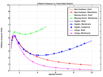
In the associated text field, type Inflation pressure (kPa).
7
Locate the Axis section. Select the Manual axis limits check box.
8
In the x minimum text field, type 0.95.
9
In the x maximum text field, type 11.
10
In the y minimum text field, type 0.
11
In the y maximum text field, type 10.
Point Graph 1
1
Right-click Inflation Pressure and choose Point Graph.
2
In the Settings window for Point Graph, locate the Data section.
3
From the Dataset list, choose Study: Neo-Hookean/Solution 2 (sol2).
4
5
Locate the y-Axis Data section. In the Expression text field, type pf_s.
6
From the Unit list, choose kPa.
7
Locate the x-Axis Data section. From the Parameter list, choose Expression.
8
Click Replace Expression in the upper-right corner of the x-Axis Data section. From the menu, choose Global definitions>Parameters>stretch - Applied stretch.
9
Click to expand the Coloring and Style section. From the Color list, choose Red.
10
Click to expand the Legends section. Select the Show legends check box.
11
From the Legends list, choose Manual.
12
Point Graph 2
1
Right-click Point Graph 1 and choose Duplicate.
2
In the Settings window for Point Graph, locate the y-Axis Data section.
3
In the Expression text field, type pf_m.
4
Locate the Coloring and Style section. Find the Line markers subsection. From the Marker list, choose Circle.
5
Locate the Legends section. In the table, enter the following settings:
Point Graph 3
1
In the Model Builder window, under Results>Inflation Pressure right-click Point Graph 1 and choose Duplicate.
2
In the Settings window for Point Graph, locate the Data section.
3
From the Dataset list, choose Study: Mooney-Rivlin/Solution 3 (sol3).
4
Locate the Coloring and Style section. From the Color list, choose Green.
5
Locate the Legends section. In the table, enter the following settings:
Point Graph 4
1
In the Model Builder window, under Results>Inflation Pressure right-click Point Graph 2 and choose Duplicate.
2
In the Settings window for Point Graph, locate the Data section.
3
From the Dataset list, choose Study: Mooney-Rivlin/Solution 3 (sol3).
4
Locate the Coloring and Style section. From the Color list, choose Green.
5
Locate the Legends section. In the table, enter the following settings:
Point Graph 5
1
In the Model Builder window, under Results>Inflation Pressure right-click Point Graph 1 and choose Duplicate.
2
In the Settings window for Point Graph, locate the Data section.
3
From the Dataset list, choose Study: Ogden/Solution 4 (sol4).
4
Locate the Coloring and Style section. From the Color list, choose Blue.
5
Locate the Legends section. In the table, enter the following settings:
Point Graph 6
1
In the Model Builder window, under Results>Inflation Pressure right-click Point Graph 2 and choose Duplicate.
2
In the Settings window for Point Graph, locate the Data section.
3
From the Dataset list, choose Study: Ogden/Solution 4 (sol4).
4
Locate the Coloring and Style section. From the Color list, choose Blue.
5
Locate the Legends section. In the table, enter the following settings:
Point Graph 7
1
Right-click Point Graph 6 and choose Duplicate.
2
In the Settings window for Point Graph, locate the y-Axis Data section.
3
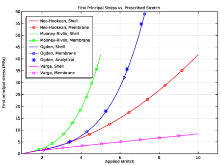
In the Expression text field, type 2*(H/Ri)*((6.3e5[Pa]*(stretch^(1.3-3)-stretch^(-2*1.3-3)))+(0.012e5[Pa]*(stretch^(5-3)-stretch^(-2*5-3)))-(0.1e5[Pa]*(stretch^(-2-3)-stretch^(2*2-3)))).
4
Locate the Coloring and Style section. Find the Line style subsection. From the Line list, choose None.
5
Find the Line markers subsection. From the Marker list, choose Asterisk.
6
In the Number text field, type 12.
7
Locate the Legends section. In the table, enter the following settings:
Point Graph 8
1
In the Model Builder window, under Results>Inflation Pressure right-click Point Graph 1 and choose Duplicate.
2
In the Settings window for Point Graph, locate the Data section.
3
From the Dataset list, choose Study: Varga/Solution 5 (sol5).
4
Locate the Coloring and Style section. From the Color list, choose Magenta.
5
Locate the Legends section. In the table, enter the following settings:
Point Graph 9
1
In the Model Builder window, under Results>Inflation Pressure right-click Point Graph 2 and choose Duplicate.
2
In the Settings window for Point Graph, locate the Data section.
3
From the Dataset list, choose Study: Varga/Solution 5 (sol5).
4
Locate the Coloring and Style section. From the Color list, choose Magenta.
5
Locate the Legends section. In the table, enter the following settings:
6
In the Inflation Pressure toolbar, click  Plot.
Inflation Pressure
To reproduce Figure 4, proceed as follows.
First Principal Stress
1
In the Model Builder window, right-click Inflation Pressure and choose Duplicate.
2
In the Settings window for 1D Plot Group, type First Principal Stress in the Label text field.
3
Locate the Title section. In the Title text area, type First Principal Stress vs. Prescribed Stretch.
4
Locate the Plot Settings section. In the y-axis label text field, type First principal stress (MPa).
5
Locate the Axis section. In the y maximum text field, type 60.
6
Locate the Legend section. From the Position list, choose Upper left.
Point Graph 1
1
In the Model Builder window, expand the First Principal Stress node, then click Point Graph 1.
2
In the Settings window for Point Graph, locate the y-Axis Data section.
3
In the Expression text field, type mat1_xdim.atxd1(shell.d/2,mean(shell.sp1)).
4
From the Unit list, choose MPa.
Point Graph 2
1
In the Model Builder window, click Point Graph 2.
2
In the Settings window for Point Graph, locate the y-Axis Data section.
3
In the Expression text field, type mbrn.sp1.
4
From the Unit list, choose MPa.
Point Graph 3
1
In the Model Builder window, click Point Graph 3.
2
In the Settings window for Point Graph, locate the y-Axis Data section.
3
In the Expression text field, type mat1_xdim.atxd1(shell.d/2,mean(shell.sp1)).
4
From the Unit list, choose MPa.
Point Graph 4
1
In the Model Builder window, click Point Graph 4.
2
In the Settings window for Point Graph, locate the y-Axis Data section.
3
In the Expression text field, type mbrn.sp1.
4
From the Unit list, choose MPa.
Point Graph 5
1
In the Model Builder window, click Point Graph 5.
2
In the Settings window for Point Graph, locate the y-Axis Data section.
3
In the Expression text field, type mat1_xdim.atxd1(shell.d/2,mean(shell.sp1)).
4
From the Unit list, choose MPa.
Point Graph 6
1
In the Model Builder window, click Point Graph 6.
2
In the Settings window for Point Graph, locate the y-Axis Data section.
3
In the Expression text field, type mbrn.sp1.
4
From the Unit list, choose MPa.
Point Graph 7
1
In the Model Builder window, click Point Graph 7.
2
In the Settings window for Point Graph, locate the y-Axis Data section.
3
In the Expression text field, type ((6.3e5[Pa]*(stretch^(1.3)-stretch^(-2*1.3)))+(0.012e5[Pa]*(stretch^(5)-stretch^(-2*5)))-(0.1e5[Pa]*(stretch^(-2)-stretch^(2*2)))).
4
From the Unit list, choose MPa.
Point Graph 8
1
In the Model Builder window, click Point Graph 8.
2
In the Settings window for Point Graph, locate the y-Axis Data section.
3
In the Expression text field, type mat1_xdim.atxd1(shell.d/2,mean(shell.sp1)).
4
From the Unit list, choose MPa.
Point Graph 9
1
In the Model Builder window, click Point Graph 9.
2
In the Settings window for Point Graph, locate the y-Axis Data section.
3
In the Expression text field, type mbrn.sp1.
4
From the Unit list, choose MPa.
5
In the First Principal Stress toolbar, click  Plot.
Finally, to reproduce Figure 5, proceed as follows.
Deformed Thickness
1
In the Home toolbar, click  Add Plot Group and choose 1D Plot Group.
2
In the Settings window for 1D Plot Group, type Deformed Thickness in the Label text field.
3
Locate the Data section. From the Dataset list, choose Study: Neo-Hookean/Solution 2 (sol2).
4
Locate the Title section. From the Title type list, choose Manual.
5
In the Title text area, type Comparison of Deformed Thickness.
6
Locate the Plot Settings section. Select the y-axis label check box.
7
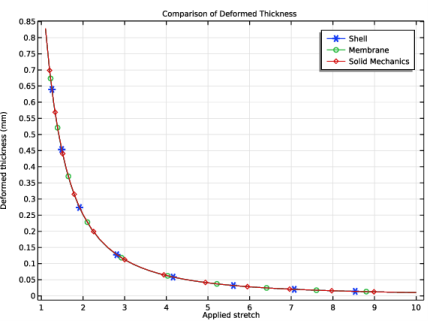
In the associated text field, type Deformed thickness (mm).
Point Graph 1
1
Right-click Deformed Thickness and choose Point Graph.
2
3
In the Settings window for Point Graph, locate the y-Axis Data section.
4
In the Expression text field, type mat1_xdim.atxd1(shell.d/2,mean(shell.ddef)).
5
From the Unit list, choose mm.
6
Locate the x-Axis Data section. From the Parameter list, choose Expression.
7
Click Replace Expression in the upper-right corner of the x-Axis Data section. From the menu, choose Global definitions>Parameters>stretch - Applied stretch.
8
Locate the Coloring and Style section. Find the Line markers subsection. From the Marker list, choose Cycle.
9
Locate the Legends section. Select the Show legends check box.
10
From the Legends list, choose Manual.
11
Point Graph 2
1
Right-click Point Graph 1 and choose Duplicate.
2
In the Settings window for Point Graph, locate the y-Axis Data section.
3
In the Expression text field, type mbrn.ddef.
4
Locate the Coloring and Style section. Find the Line markers subsection. In the Number text field, type 10.
5
Locate the Legends section. In the table, enter the following settings:
Global 1
1
In the Model Builder window, right-click Deformed Thickness and choose Global.
2
In the Settings window for Global, locate the y-Axis Data section.
3
4
Click Replace Expression in the upper-right corner of the x-Axis Data section. From the menu, choose Global definitions>Parameters>stretch - Applied stretch.
5
Click to expand the Coloring and Style section. Find the Line markers subsection. From the Marker list, choose Diamond.
6
In the Number text field, type 12.
7
Click to expand the Legends section. From the Legends list, choose Manual.
8
9
In the Deformed Thickness toolbar, click  Plot.