Arterial Wall Viscoelasticity

Arteries are blood vessels that carry freshly oxygenated blood from the heart throughout the rest of the body. The Holzapfel–Gasser–Ogden (HGO) model proposes a mechanical description of the young healthy arteries in Ref. 1 based on anisotropic hyperelastic properties, which is implemented in the Arterial Wall Mechanics example. Here we study the dynamic behavior of the artery, based on Ref. 2 and calculate the time-dependent response given a sudden axial stretching.

Model Definition

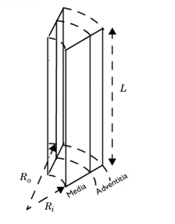
The geometry, physics interface, and material models are the same as in the example Arterial Wall Mechanics, see also Figure 1.

Figure 1: Carotid artery section made of a media layer and an adventitia layer.

The two modeled layers (media and adventitia) are described by the anisotropic HGO hyperelastic material model:

Only the media layer includes viscoelastic behavior. The generalized Maxwell viscoelastic model is used to represent relaxations time at different time-scales (Ref. 2):

(1)

For each branch of the generalized Maxwell model, the viscoelastic stress follows the equation:

where τm is the relaxation time and βm is the energy factor per branch. Applying a variable change qm = βmSiso − Qm gives

(2)

In this example, a generalized Maxwell viscoelastic model with five branches is used with the following values taken from Ref. 2:


Branch	Energy factor	Relaxation time
1	0.3353	0.001 s
2	0.286	0.01 s
3	0.298	0.1 s
4	0.285	1 s
5	0.348	10 s

The artery is first loaded with an internal pressure of 100 mmHg and an initial axial stretch of 1.5. After initialization, the stretch is increased to 1.7 and the viscoelastic relaxation is calculated.

Results and Discussion

The total force is computed by integrating the axial stress on the top section surface. The plot shown in Figure 2 is similar to the force relaxation presented in Ref. 2. The force relaxes almost linearly from 10-3 s to 10 s due to the wide range of relaxation times.

Moreover, Figure 3 shows the evolution of total viscoelastic stress and viscoelastic stress for each branch over time. The viscoelastic stress for the branches is calculated with the expression

. The viscoelastic stress relaxes from its initial value to zero.

Figure 2: Relaxation of the axial force after stretching.

Figure 3: Variation of viscoelastic stress. Both the total stress and the stress in each branch is shown.

Notes About the COMSOL Implementation

A stationary study step is needed to prestress the artery with initial pressure and stretch. As this initial state is assumed to be a steady-state, the static stiffness in node must be set to . This ensures that the viscoelastic model has no effects in the stationary step.

References

1. G. Holzapfel, T. Gasser, and R. Ogden, “A New Constitutive Framework for Arterial Wall Mechanics and a Comparative Study of Material Models,” J. Elasticity, vol. 61, pp. 1–48, 2000.

2. G.A. Holzapfel, T.C. Gasser, M. Stadler, “A Structural Model for the Viscoelastic Behavior of Arterial Walls: Continuum Formulation and Finite Element Analysis”, European Journal of Mechanics A/Solid, vol.21, pp. 441–463, 2002

Nonlinear_Structural_Materials_Module/Viscoelasticity/arterial_wall_viscoelasticity

Modeling Instructions

From the menu, choose .

From the Application Libraries root, browse to the folder Nonlinear_Structural_Materials_Module/Hyperelasticity and double-click the file arterial_wall_mechanics.mph.

Global Definitions

Parameters 1

Set the parameters used for loads and constraints in the time dependent study. Parameter t is the time, and is needed to define the prescribed displacement in the stationary study step.

In the window, under click .

In the window for , locate the section.

In the table, enter the following settings:


Name	Expression	Value	Description
p_i	100[mmHg]	13332 Pa	Internal pressure
lambda_z	1.7	1.7	Axial stretch
lambda_z0	1.5	1.5	Initial axial stretch
t	0[s]	0 s	Time

Create a step function to apply the stretch in the time-dependent study.

Step 1 (step1)

In the toolbar, click

and choose .

In the window for , type lambda in the text field.

Locate the section. In the text field, type 5e-6.

In the text field, type lambda_z0.

In the text field, type lambda_z.

Click to expand the section. In the text field, type 1e-5.

Click

Component 1 (comp1)

In the window, expand the node.

Solid Mechanics (solid)

Hyperelastic Material 1

Add a generalized Maxwell viscoelasticity model according to Ref. 1.

In the window, expand the node, then click .

Viscoelasticity 1

In the toolbar, click

and choose .

Select Domain 1 only.

In the window for , locate the section.

Click

four times.

In the table, enter the following settings:


Branch	Energy factor (1)	Relaxation time (s)
1	0.353	0.001
2	0.286	0.01
3	0.298	0.1
4	0.285	1
5	0.348	10

Prescribed Displacement 2

In the window, under right-click and choose .

In the window for , locate the section.

In the u 0 z text field, type (lambda(t[1/s])-1)*L.

Definitions

Integration 1 (intop1)

In the toolbar, click

and choose .

In the window for , locate the section.

From the list, choose .

Select Boundaries 3 and 6 only.

Mesh 2

In the toolbar, click

Mapped 1

In the toolbar, click

Distribution 1

In the window, right-click and choose .

Select Boundaries 2 and 3 only.

In the window for , locate the section.

From the list, choose .

In the text field, type 20.

In the text field, type 10.

Select the check box.

Distribution 2

In the window, right-click and choose .

Select Boundary 5 only.

In the window for , locate the section.

In the text field, type 8.

In the window, right-click and choose .

Add a new study. The first stationary step is used to prestress the artery with a stretch and an internal pressure. Select in the node, so the viscoelastic effect is disabled. The time-dependent step is used to compute the dynamic response to an additional stretch.

Add Study

In the toolbar, click

to open the window.

Go to the window.

Find the subsection. In the tree, select .

Find the subsection. In the table, clear the check boxes for , , , and .

Click in the window toolbar.

In the toolbar, click

to close the window.

Study 2

Step 1: Stationary

In the window for , click to expand the section.

Select the check box.

Click

In the table, enter the following settings:


Parameter name	Parameter value list	Parameter unit
p_i (Internal pressure)	range(0,10,100)	mmHg

Time Dependent

In the toolbar, click

and choose .

In this study clear the check box for all interfaces.

In the window for , locate the section.

In the text field, type range(0,0.5e-6,9.5e-6) 10^{range(-5,0.2,2.4)}.

From the list, choose .

In the text field, type 0.001.

Click to expand the section. Find the subsection. From the list, choose .

From the list, choose .

Solution 2 (sol2)

In the toolbar, click

In the window, expand the node, then click .

In the window for , click to expand the section.

From the list, choose .

In the window, click .

In the window for , locate the section.

Clear the check box.

In the toolbar, click

Results

Study 2/Solution 2 (sol2)

In the window, expand the node, then click .

In the window for , locate the section.

From the list, choose .

Integrate the axial stress on the top surfaces to calculate the reaction force and reproduce Figure 2.

Force Relaxation

In the toolbar, click

and choose .

In the window for , type Force Relaxation in the text field.

Locate the section. From the list, choose .

From the list, choose .

In the text field, type 10^{range(-5,0.2,2.4)}.

Click the

button in the toolbar.

In the toolbar, click

Global 1

Right-click and choose .

In the window for , locate the section.

In the table, enter the following settings:


Expression	Unit	Description
intop1(solid.sz)	mN	Axial Force

In the toolbar, click

Add a new plot group to plot viscoelastic stress and reproduce Figure 3.

Viscoelastic Stress

In the toolbar, click

and choose .

In the window for , type Viscoelastic Stress in the text field.

Locate the section. From the list, choose .

From the list, choose .

In the text field, type 10^{range(-5,0.2,2.4)}.

Click to expand the section. From the list, choose .

In the text area, type Radial viscoelastic stress.

Locate the section. Select the check box.

In the associated text field, type Viscoelastic stress (N/m^2).

Locate the section. From the list, choose .

Point Graph 1

Right-click and choose .

Select Point 1 only.

In the window for , click in the upper-right corner of the section. From the menu, choose .

Click to expand the section. Select the check box.

From the list, choose .

In the table, enter the following settings:


Legends
Total Viscoelastic Stress

Point Graph 2

Right-click and choose .

In the window for , locate the section.

In the text field, type solid.hmm1.vis1.betavm1*solid.Sliso11-solid.hmm1.vis1.qm1_11.

Locate the section. In the table, enter the following settings:


Legends
Branch 1

Duplicate the point graph four times and change properties according to the table:


Point graph	Expression of y-Axis Data	Legends
Point Graph 3	solid.hmm1.vis1.betavm2*solid.Sliso11-solid.hmm1.vis1.qm2_11	Branch 2
Point Graph 4	solid.hmm1.vis1.betavm3*solid.Sliso11-solid.hmm1.vis1.qm3_11	Branch 3
Point Graph 5	solid.hmm1.vis1.betavm4*solid.Sliso11-solid.hmm1.vis1.qm4_11	Branch 4
Point Graph 6	solid.hmm1.vis1.betavm5*solid.Sliso11-solid.hmm1.vis1.qm5_11	Branch 5