Transport and Adsorption

This example demonstrates how you can model phenomena defined in different dimensions (2D and 1D in this example) in a fully coupled manner using COMSOL Multiphysics.

In this particular case, the model involves a small parallel-plate reactor with a catalytic surface. Similar applications where surface processes are of critical importance include biochip devices and a semiconductor components.

When modeling chemical reactions the reaction rates are commonly functions of the concentrations of the reactants in the phase that transports the chemicals. However, for surface reactions it is also necessary to account for the surface concentrations of the active sites and surface adsorbed species. The mass balances in the bulk of the reactor must therefore be coupled to the mass balances for species, present only at the surface of the device.

Model Definition

The first approximation you can make is to reduce the 3D geometry to 2D, which is reasonable if the variations in concentration are small along the depth of the domain. Figure 1 shows how the 2D model domain is related to the full 3D reactor geometry.

Figure 1: The modeled domain is a parallel plate reactor with an active surface where you want to model the concentration of surface species. A denotes molecular species dissolved in gas and As the same species adsorbed on the surface.

Model Equations

The adsorption/desorption reaction at the surface is described by

where kf and kr are forward and reverse rate constants. A and As are the molecular species in the gas and adsorbed on active sites on the surface, respectively.

Let θ be the fraction of active sites occupied by adsorbed molecules. The fraction of free sites is then 1 − θ. Langmuir derived that the rate of desorption of molecules, rdes (mol/(m2·s)), is proportional to θ and equal to krθ where kr is a constant at constant temperature. Furthermore, the rate of adsorption of molecules is proportional to both the fraction of free surface sites, 1 − θ, and to the rate of which molecules strike the surface. The collision rate is in turn directly proportional the partial pressure of the species, pA (Pa). The rate of adsorption in mol/(m2·s) is thus rads = kfpA(1 − θ), where kf is a constant at constant temperature.

To set up transport and reaction equations in terms of c (bulk gas concentration of A in mol/m3) and cs (surface concentration of A in mol/m2), make the following substitutions:

where

•

Γs is the total surface concentration of active sites (mol/m2)

•

R is the gas constant (J/(mol·K))

•

T is temperature (K)

which yields

(1)

and

where

•

kdes = kr/Γs is the rate constant for the desorption reaction (m3/(mol·s))

•

kads = kfRT/Γs is the rate constant for the adsorption reaction (1/s)

The surface concentration is in moles per unit surface.

The material balance for the surface, including surface diffusion and the reaction rate expression for the formation of the adsorbed species, cs, is:

where Ds represents surface diffusivity. This gives the following equation for the transport and reaction on the surface:

(2)

Equation 2 defines the units of the rate constants kads and kdes. The initial condition is that the concentration of adsorbed species is zero at the beginning of the process:

The equation for the surface-reaction expression includes the concentration of the bulk species, c, at the position of the catalyst surface. Thus you must solve the equation for the surface reaction in combination with the mass balance in the bulk. The coupling between the mass balance in the bulk and the surface is obtained as a boundary condition in the bulk’s mass balance. This condition sets the flux of c at the boundary equal to the rate of the surface reaction and is presented below. The transport in the bulk of the reactor is described by a convection-diffusion equation:

(3)

The initial condition sets the concentration in the bulk at t = 0:

In the above equation, D denotes the diffusivity of the reacting species, c is its concentration, and u is the velocity. In this case, the velocity in the x direction equals 0 while the velocity in the y direction comes from the analytical expression for fully developed laminar flow between two parallel plates:

Here, δ is the distance between the plates, vmax is the maximum local velocity, and x = 0 at the left boundary of the 2D model geometry shown on the right in Figure 1.

Boundary Conditions

The boundary conditions for the surface species are insulating conditions according to:

(4)

For the bulk, the boundary condition at the active surface couples the rate of the reaction at the surface with the flux of the reacting species and the concentration of the adsorbed species and bulk species:

(5)

The other boundary conditions for the bulk problem are:

•

Inlet: c = c0

•

Outlet: n · (−D∇c + cu) = n · cu

•

Insulation: n · (−D∇c + cu) = 0

Notes About the COMSOL Implementation

This example deals with a phenomenon (convection-diffusion) occurring in a 2D domain coupled to another phenomenon (diffusion-reaction) occurring only on a part of this domain’s 1D boundary. Model the 2D equation (Equation 3) using a Transport of Diluted Species interface and the 1D equation (Equation 2) with a General Form Boundary PDE interface on the active-surface boundary. The two interfaces are coupled through the surface reaction rate expression on the right-hand side of Equation 2, which becomes a flux in the boundary condition Equation 5 for Equation 3. The Neumann condition Equation 4 is a natural boundary condition, which means that you do not need to impose it explicitly.

Results and Discussion

The plot in Figure 2 shows the concentration, c, of the reacting species in the 2D domain after 2 seconds of operation. The reaction is very fast and has almost reached steady state in that time frame. Figure 3, which displays the concentration along a vertical cross section of the active surface, shows that the concentration distribution exhibits edge effects at both ends of the catalyst. The higher concentration near y = 0 is easy to explain because this is the position closest to the inlet, and this end is therefore continuously supplied with fresh reactant. The increase in concentration at the end closer to the outlet is due to diffusion; the edge of the surface can receive diffusion in all directions within a 90° angle without having to compete for the reactant supply with other parts of the catalysts. This effect also appears at the edge close to the inlet.

Figure 2: Concentration of the reacting species, c, after 2 seconds of operation (t = 2 s).

Figure 3: Concentration of the reacting species along the active surface at t = 2 s.

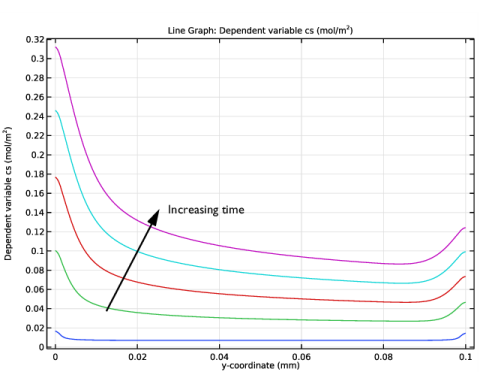
The concentration of adsorbed species, cs, shows a similar spatial distribution. However, while the concentration of the reactant decreases with time, the concentration of adsorbed species increases. You can also see that the slight spatial diffusion evens out the concentration gradients somewhat; see Figure 4.

Figure 4: The concentration of adsorbed species increases with time. The edge effect appears at both edges due to the increased supply of reactants. This figure displays the concentration after 0.05, 0.5, 1.0, 1.5, and 2.0 s.

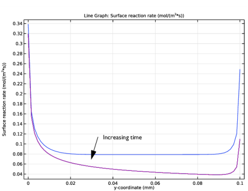
The concentration of gas phase species at the surface decreases while the surface concentration of the adsorbed species increases with time. This implies that the adsorption rate decreases with time. You can see this effect in Figure 5, which also shows that after 0.5 s the reaction rate almost reaches steady-state. The upper curve shows the reaction rate after 0.05 s, while the lower curve represents the curves for 0.5, 1.0, 1.5, and 2.0 s, which are all on top of each other.

Figure 5: Surface reaction rate at the active surface. The largest reaction rate is obtained initially and is at the edges of the active surface. The reaction process almost reaches steady state at 0.5 s.

COMSOL_Multiphysics/Chemical_Engineering/transport_and_adsorption

Modeling Instructions

From the menu, choose .

New

In the window, click

Model Wizard

In the window, click

In the tree, select .

Click .

In the tree, select .

Click .

In the table, enter the following settings:


cs

Click

In the tree, select .

Click

Global Definitions

A set of model parameters is available in a text file.

Parameters 1

In the window, under click .

In the window for , locate the section.

Click

Browse to the model’s Application Libraries folder and double-click the file transport_and_adsorption_parameters.txt.

Geometry 1

In the window, under click .

In the window for , locate the section.

From the list, choose .

Rectangle 1 (r1)

In the toolbar, click

In the window for , locate the section.

In the text field, type 0.1.

In the text field, type 0.3.

Locate the section. In the text field, type -0.1.

Click

Point 1 (pt1)

In the toolbar, click

In the window for , locate the section.

In the text field, type 0.1.

Click

Point 2 (pt2)

In the toolbar, click

In the window for , locate the section.

In the text field, type 0.1.

Click

Click the

button in the toolbar.

Definitions

Variables 1

In the toolbar, click

and choose .

In the window for , locate the section.

From the list, choose .

Select Boundary 5 only.

Locate the section. In the table, enter the following settings:


Name	Expression	Description
R	k_adsc(Gamma_s-cs)-k_des*cs	Surface reaction rate

Variables 2

In the toolbar, click

and choose .

In the window for , locate the section.

From the list, choose .

Select Domain 1 only.

Locate the section. In the table, enter the following settings:


Name	Expression	Unit	Description
v_lam	v_max(1-((x-0.5delta)/(0.5*delta))^2)	m/s	Inlet velocity profile

Transport of Diluted Species (tds)

Transport Properties 1

In the window, under click .

In the window for , locate the section.

In the Dc text field, type D.

Locate the section. Specify the u vector as


0	x
v_lam	y

Initial Values 1

In the window, click .

In the window for , locate the section.

In the c text field, type c0.

Concentration 1

In the toolbar, click

and choose .

Select Boundary 2 only.

In the window for , locate the section.

Select the check box.

In the c0,c text field, type c0.

Flux 1

In the toolbar, click

and choose .

Select Boundary 5 only.

In the window for , locate the section.

Select the check box.

In the J0,c text field, type -R.

Outflow 1

In the toolbar, click

and choose .

Select Boundary 3 only.

Symmetry 1

In the toolbar, click

and choose .

Select Boundaries 1, 4, and 6 only.

General Form Boundary PDE (gb)

Next, set up the equation and boundary conditions for the surface concentration, cs.

In the window, under click .

In the window for , locate the section.

From the list, choose .

Click

Select Boundary 5 only.

Locate the section. Click

In the table, enter the following settings:


Dependent variable quantity	Unit
Custom unit	mol/m^2

In the table, enter the following settings:


Source term quantity	Unit
Custom unit	mol/(m^2*s)

General Form PDE 1

In the window, under click .

In the window for , click to expand the section.

Comparing this equation with Equation 1 in the Model Definition section leads to the following settings:

Locate the section. Specify the Γ vector as


-csTx*Ds	x
-csTy*Ds	y

Here, csTx and csTy refer to the components of the gradient nabla c_s restricted to the plane tangential to the boundary where the interface is defined, that is, Boundary 5. Because this boundary is parallel to the y-axis, only csTy is nonzero in this case.

Locate the section. In the f text field, type R.

Initial Values 1

The default initial value, 0, for the surface concentration applies for this model, so you do not need to set it explicitly.

Mesh 1

Free Triangular 1

In the toolbar, click

Size 1

Right-click and choose .

In the window for , locate the section.

From the list, choose .

Select Boundary 5 only.

Locate the section. Click the button.

Locate the section. Select the check box.

In the associated text field, type 1.5[um].

Click

Study 1

Step 1: Time Dependent

In the window, under click .

In the window for , locate the section.

In the text field, type range(0,0.05,2).

In the toolbar, click

Results

Concentration species in reactor

In the window for , type Concentration species in reactor in the text field.

Click the

button in the toolbar.

In the toolbar, click

The first default plot shows the concentration of the reacting species at the end of the simulation interval, t = 2 s.

Concentration reacting species along active surface

Create a plot of the final concentration at the reacting surface.

In the toolbar, click

and choose .

In the window for , type Concentration reacting species along active surface in the text field.

Locate the section. From the list, choose .

In the list, select .

Line Graph 1

Right-click and choose .

Select Boundary 5 only.

In the window for , click in the upper-right corner of the section. From the menu, choose .

In the toolbar, click

The plot should look like that in Figure 3.

Concentration reacting species along active surface

Proceed to reproduce the plot in Figure 4 showing the concentration of adsorbed species at selected times. You can use the plot group you just created as the starting point.

Concentration adsorbed species along active surface

In the window, right-click and choose .

In the window for , type Concentration adsorbed species along active surface in the text field.

Locate the section. In the list, choose , , , , and .

Line Graph 1

In the window, expand the node, then click .

In the window for , click in the upper-right corner of the section. From the menu, choose .

In the toolbar, click

Finally, reproduce the plot in Figure 5 of the surface reaction rate at the same times. Again, use the previous plot group as the starting point.

Surface reaction rate along active surface

In the window, right-click and choose .

In the window for , type Surface reaction rate along active surface in the text field.

Line Graph 1

In the window, expand the node, then click .

In the window for , click in the upper-right corner of the section. From the menu, choose .

In the toolbar, click

Concentration species in reactor

Click the

button in the toolbar.

In the window, click .

In the toolbar, click

Rename and use a tube line type to illustrate the adsorbed species concentration over the 2D geometry.

Concentration adsorbed species at active surface

In the window, under click .

In the window for , type Concentration adsorbed species at active surface in the text field.

Line 1

In the window, expand the node, then click .

In the window for , locate the section.

From the list, choose .

Select the check box.

In the associated text field, type 0.005.

Click the

button in the toolbar.

In the toolbar, click