|
|
|
|
•
|
|
1
|
|
2
|
|
3
|
|
4
|
|
1
|
|
2
|
|
3
|
|
4
|
|
5
|
|
6
|
|
1
|
|
2
|
|
3
|
|
4
|
|
5
|
|
1
|
|
2
|
|
3
|
|
4
|
|
5
|
|
1
|
|
2
|
|
1
|
|
2
|
|
1
|
|
2
|
In the Show More Options dialog box, in the tree, select the check box for the node Study>Reduced-Order Modeling.
|
|
3
|
Click OK.
|
|
4
|
|
1
|
|
1
|
|
2
|
|
3
|
|
4
|
|
5
|
|
1
|
|
2
|
|
3
|
|
1
|
|
3
|
|
4
|
|
1
|
|
3
|
In the Settings window for Flux/Source, click to expand the Boundary Absorption/Impedance Term section.
|
|
4
|
|
1
|
|
2
|
|
3
|
|
4
|
|
5
|
|
1
|
|
2
|
|
3
|
|
1
|
In the Model Builder window, expand the Component 1 (comp1)>Definitions>Thermostat position 1 node, then click Point Probe Expression 1 (ppb1).
|
|
2
|
|
1
|
In the Model Builder window, expand the Component 1 (comp1)>Definitions>Thermostat position 2 node, then click Point Probe Expression 1 (ppb2).
|
|
2
|
|
1
|
In the Model Builder window, under Component 2 (comp2) right-click Definitions and choose Variables.
|
|
2
|
|
1
|
|
2
|
|
3
|
|
4
|
|
5
|
|
1
|
|
2
|
|
1
|
|
2
|
|
1
|
|
2
|
|
3
|
|
4
|
|
5
|
Locate the Reinitialization section. In the table, enter the following settings:
|
|
1
|
|
2
|
|
3
|
|
4
|
Locate the Reinitialization section. In the table, enter the following settings:
|
|
1
|
In the Model Builder window, under Global Definitions>Reduced-Order Modeling click Global Reduced Model Inputs 1.
|
|
2
|
|
1
|
|
2
|
|
3
|
|
4
|
|
5
|
|
1
|
|
2
|
|
3
|
|
4
|
|
1
|
|
2
|
|
3
|
|
4
|
|
5
|
|
6
|
|
7
|
|
1
|
|
2
|
|
3
|
In the Settings window for Table, type Full model outputs Tset = 20 degrees C, position 1 in the Label text field.
|
|
1
|
|
2
|
|
3
|
|
4
|
|
1
|
|
2
|
|
3
|
|
4
|
|
1
|
|
2
|
|
3
|
|
4
|
Locate the Physics and Variables Selection section. In the table, clear the Solve for check box for Events (ev).
|
|
5
|
|
1
|
|
2
|
|
3
|
|
4
|
|
1
|
|
2
|
|
3
|
|
1
|
|
2
|
|
3
|
|
4
|
|
5
|
|
6
|
Locate the Outputs section. In the table, enter the following settings:
|
|
7
|
Locate the Model Control Inputs section. In the table, set up the training values: change the value of Tout to 293.15 and HeatState to 1.
|
|
8
|
|
1
|
|
2
|
|
3
|
|
1
|
|
2
|
|
3
|
|
1
|
|
1
|
|
2
|
|
3
|
|
1
|
|
2
|
|
3
|
|
1
|
|
2
|
|
3
|
|
4
|
|
5
|
|
1
|
|
2
|
|
3
|
|
4
|
|
5
|
|
6
|
|
7
|
|
8
|
|
9
|
|
10
|
|
11
|
|
12
|
|
1
|
|
2
|
|
3
|
|
4
|
|
5
|
|
6
|
|
1
|
|
2
|
In the Settings window for Table, type Reduced Model outputs, 6 modes Tset = 20 degrees C, position 1 in the Label text field.
|
|
1
|
|
2
|
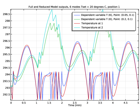
In the Settings window for 1D Plot Group, type Full and Reduced Model outputs, 6 modes Tset = 20 degrees C, position 1 in the Label text field.
|
|
3
|
|
4
|
In the Title text area, type Full and Reduced Model outputs, 6 modes Tset = 20 degrees C, position 1.
|
|
1
|
In the Model Builder window, expand the Full and Reduced Model outputs, 6 modes Tset = 20 degrees C, position 1 node, then click Probe Table Graph 1.
|
|
2
|
|
3
|
Locate the Data section. From the Table list, choose Full model outputs Tset = 20 degrees C, position 1.
|
|
1
|
|
2
|
In the Settings window for Table Graph, type Reduced model output table graph in the Label text field.
|
|
3
|
Locate the Data section. From the Table list, choose Reduced Model outputs, 6 modes Tset = 20 degrees C, position 1.
|
|
1
|
In the Model Builder window, click Full and Reduced Model outputs, 6 modes Tset = 20 degrees C, position 1.
|
|
2
|
|
1
|
|
2
|
|
3
|
|
1
|
|
2
|
|
3
|
|
4
|
|
1
|
|
2
|
In the Settings window for Table, type Reduced Model outputs, 30 modes Tset = 20 degrees C, position 1 in the Label text field.
|
|
1
|
|
2
|
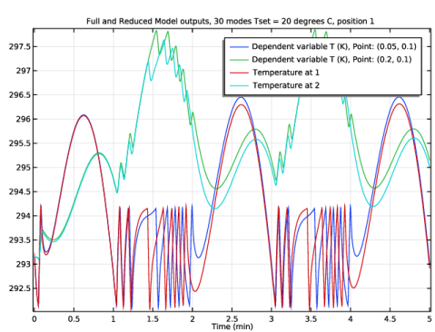
In the Settings window for 1D Plot Group, type Full and Reduced Model outputs, 30 modes Tset = 20 degrees C, position 1 in the Label text field.
|
|
3
|
|
4
|
In the Title text area, type Full and Reduced Model outputs, 30 modes Tset = 20 degrees C, position 1.
|
|
1
|
In the Model Builder window, expand the Full and Reduced Model outputs, 30 modes Tset = 20 degrees C, position 1 node, then click Probe Table Graph 1.
|
|
2
|
|
3
|
Locate the Data section. From the Table list, choose Full model outputs Tset = 20 degrees C, position 1.
|
|
1
|
|
2
|
In the Settings window for Table Graph, type Reduced model output table graph in the Label text field.
|
|
3
|
Locate the Data section. From the Table list, choose Reduced Model outputs, 30 modes Tset = 20 degrees C, position 1.
|
|
1
|
In the Model Builder window, click Full and Reduced Model outputs, 30 modes Tset = 20 degrees C, position 1.
|
|
2
|
In the Full and Reduced Model outputs, 30 modes Tset = 20 degrees C, position 1 toolbar, click
 |
|
1
|
|
2
|
|
3
|
|
1
|
|
2
|
In the Settings window for Table, type Reduced Model outputs, 30 modes Tset = 300 K, position 1 in the Label text field.
|
|
1
|
|
2
|
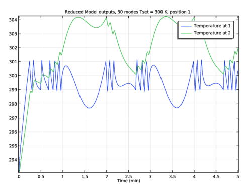
In the Settings window for 1D Plot Group, type Reduced Model outputs, 30 modes Tset = 300 K, position 1 in the Label text field.
|
|
3
|
|
4
|
|
1
|
In the Model Builder window, expand the Reduced Model outputs, 30 modes Tset = 300 K, position 1 node, then click Probe Table Graph 1.
|
|
2
|
|
3
|
|
1
|
|
2
|
|
3
|
|
1
|
|
2
|
In the Settings window for Table, type Reduced Model outputs, 30 modes Tset = 300 K, position 2 in the Label text field.
|
|
1
|
|
2
|
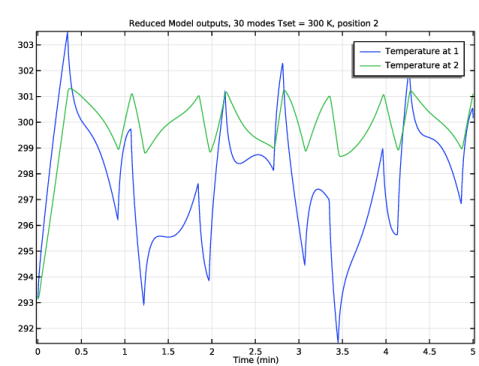
In the Settings window for 1D Plot Group, type Reduced Model outputs, 30 modes Tset = 300 K, position 2 in the Label text field.
|
|
3
|
|
4
|
|
1
|
In the Model Builder window, expand the Reduced Model outputs, 30 modes Tset = 300 K, position 2 node, then click Probe Table Graph 1.
|
|
2
|
|
3
|
|
1
|
|
2
|
|
3
|
|
1
|
|
2
|
|
3
|
|
4
|
|
5
|
|
6
|
|
7
|
|
8
|
|
9
|
|
1
|
|
2
|
In the Settings window for Table, type Full Model outputs, Tset = 300 K, position 2 in the Label text field.
|
|
1
|
|
2
|
|
3
|
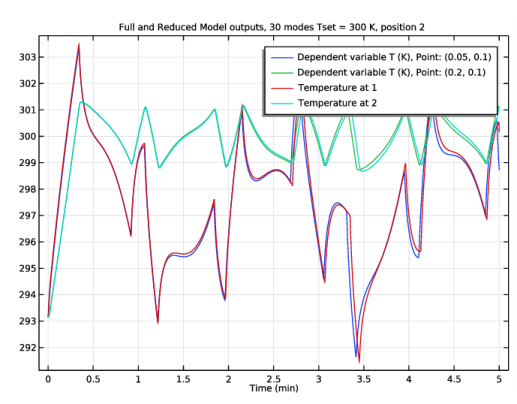
In the Settings window for 1D Plot Group, type Full and Reduced Model outputs, 30 modes Tset = 300 K, position 2 in the Label text field.
|
|
4
|
|
5
|
|
1
|
In the Model Builder window, under Results>Full and Reduced Model outputs, 30 modes Tset = 300 K, position 2 click Probe Table Graph 1.
|
|
2
|
|
3
|
|
1
|
|
2
|
In the Settings window for Table Graph, type Reduced model output table graph in the Label text field.
|
|
3
|
Locate the Data section. From the Table list, choose Reduced Model outputs, 30 modes Tset = 300 K, position 2.
|