Shell Diffusion in a Tank

You are viewing the documentation for an older COMSOL version. The latest version is available here.

PDF

Shell Diffusion in a Tank

A goal for many applications is to predict physics in thin structures, such as shells, without modeling the thickness of the structure. This is because large aspect ratios can cause meshing and geometry analysis problems. The model reported here demonstrates how to use the tangential derivative variables in COMSOL Multiphysics to solve partial differential equations in curved 3D shells and 2D boundaries without modeling their thickness.

Model Definition

The steel tank shown below has two pipe connections. One is grounded and the other connects to a dead current source. This model calculates the current density in the tank shell along with the potential distribution across the surface.

The fundamental equation to solve is the current conduction, or charge conservation, equation.

(1)

Here, σ is the electrical conductivity (S/m) and V is the electric potential (V).

The material is a 1 mm thick steel sheet with a conductivity of 4.032·106 S/m. You are working with a surface in 3D so there is no thickness in the model. To account for the charge conservation in Equation 1 you must multiply the current flux expression with the shell thickness d:

(2)

Figure 1 shows the potential distribution across the surface.

Figure 1: Electric potential distribution across the surface (V).

Figure 2 adds the current field as an arrow plot, showing clearly how the current collects toward the grounded connection.

Figure 2: Arrow plot of the local current field.

Figure 3: Local magnitude of the electric current density (A/m2).

The plot of the magnitude of the local current density in Figure 3 is interesting because you can use it to calculate the resistive heating in the material as an extension to the model.

Notes About the COMSOL Implementation

Model Equation 2, the current conduction equation, using a Coefficient Form Boundary PDE interface, setting the diffusion coefficient c = σd. To define the current field components use tangential derivative variables, which you access in COMSOL Multiphysics by adding a T suffix to the variable name before specifying the gradient component. So, for example, the tangential derivative (∂u/∂x)T is represented by the variable uTx.

COMSOL_Multiphysics/Equation_Based/shell_diffusion

Modeling Instructions

From the menu, choose .

In the window, click

.

1

In the window, click

.

2

In the tree, select .

3

4

In the table, enter the following settings:


V

5

6

In the tree, select .

7

Global Definitions

1

In the window, under click .

2

In the window for , locate the section.

3

In the table, enter the following settings:


Name	Expression	Value	Description
sigma	4.032e6[S/m]	4.032E6 S/m	Conductivity
d	1[mm]	0.001 m	Shell thickness

Create the geometry. To simplify this step, insert a prepared geometry sequence.

1

In the toolbar, click

.

2

Browse to the model’s Application Libraries folder and double-click the file shell_diffusion_geom_sequence.mph.

3

In the toolbar, click

.

4

button in the toolbar.

Coefficient Form Boundary PDE (cb)

1

In the window, under click .

2

In the window for , locate the section.

3

.

4

In the dialog box, type electricpotential in the text field.

5

6

In the tree, select .

7

8

In the window for , locate the section.

9

In the table, enter the following settings:


Source term quantity	Unit
Custom unit	A*m^-2

Coefficient Form PDE 1

1

In the window, under click .

2

In the window for , locate the section.

3

In the c text field, type sigma*d.

4

Locate the section. In the f text field, type 0.

These settings specify the charge conservation equation (Equation 2) for the shell surface.

Go on to set the values of the potential at the pipe connections by adding Dirichlet boundary conditions.

Dirichlet Boundary Condition 1

1

In the toolbar, click

and choose .

2

Select Edges 14, 15, 25, and 29 only.

3

In the window for , locate the section.

4

In the r text field, type 400.

Dirichlet Boundary Condition 2

1

In the toolbar, click

and choose .

2

Select Edges 40–43 only.

1

In the window, under click .

2

In the window for , locate the section.

3

From the list, choose .

4

.

In the toolbar, click

.

3D Plot Group 1

The default plot shows the potential distribution.

1

button in the toolbar.

Rotate the geometry so that you see both pipe connections. Compare the result with the plot in Figure 1.

Add an arrow surface plot of the current field as follows:

Arrow Surface 1

1

Right-click and choose .

2

In the window for , locate the section.

3

In the text field, type -sigma*VTx.

4

In the text field, type -sigma*VTy.

5

In the text field, type -sigma*VTz.

6

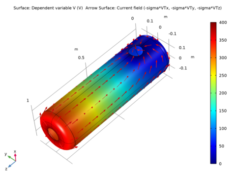
Select the check box.

7

In the associated text field, type Current field (-sigma*VTx, -sigma*VTy, -sigma*VTz).

8

Locate the section. From the list, choose .

9

In the toolbar, click

.

The plot in the window should now look like that in Figure 2.

To visualize the magnitude of the local current density, follow the steps given below.

3D Plot Group 2

1

In the toolbar, click

and choose .

2

In the window for , click to expand the section.

3

From the list, choose .

4

In the text area, type Current density (A/m<sup>2</sup>).

1

Right-click and choose .

2

In the window for , locate the section.

3

In the text field, type sigma*sqrt(VTx^2+VTy^2+VTz^2).

4

In the toolbar, click

.

5

button in the toolbar.