
|
|
|
|
1
|
|
2
|
|
3
|
Click Add.
|
|
4
|
|
5
|
In the Dependent variables table, enter the following settings:
|
|
6
|
Click
|
|
7
|
|
8
|
Click
|
|
1
|
|
2
|
|
3
|
|
1
|
|
2
|
|
1
|
|
2
|
|
4
|
|
1
|
|
2
|
|
1
|
In the Model Builder window, under Component 1 (comp1)>General Form PDE (g) click General Form PDE 1.
|
|
2
|
|
3
|
|
4
|
|
5
|
|
6
|
|
1
|
|
2
|
|
3
|
|
1
|
|
2
|
Click in the Graphics window and then press Ctrl+A to select both boundaries.
|
|
3
|
|
4
|
|
1
|
|
2
|
|
3
|
Click the Custom button.
|
|
4
|
|
5
|
|
1
|
|
2
|
|
3
|
|
4
|
|
5
|
|
1
|
|
2
|
|
3
|
|
4
|
|
5
|
|
6
|
|
1
|
|
2
|
|
1
|
|
2
|
|
3
|
|
4
|
|
5
|
|
6
|
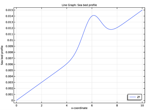
Click Replace Expression in the upper-right corner of the y-Axis Data section. From the menu, choose Component 1 (comp1)>Definitions>Variables>Zf - Sea bed profile.
|
|
7
|
|
8
|
|
10
|
|
1
|
|
2
|
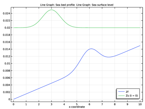
In the Settings window for Line Graph, click Replace Expression in the upper-right corner of the y-Axis Data section. From the menu, choose Component 1 (comp1)>Definitions>Variables>Zs - Sea surface level.
|
|
3
|
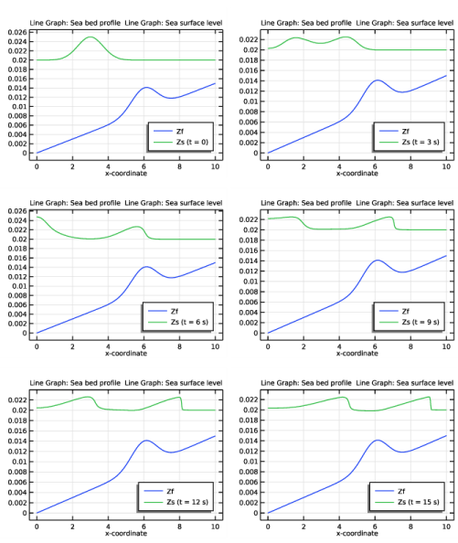
Locate the Legends section. In the table, enter the following settings:
|
|
4
|
|
5
|
|
6
|
Locate the Legends section. In the table, enter the following settings:
|
|
7
|
|
8
|
|
9
|
Locate the Legends section. In the table, enter the following settings:
|
|
10
|
|
11
|
|
12
|
Locate the Legends section. In the table, enter the following settings:
|
|
13
|
|
14
|
|
15
|
Locate the Legends section. In the table, enter the following settings:
|
|
16
|
|
17
|
|
18
|
Locate the Legends section. In the table, enter the following settings:
|
|
19
|