|
|
|


|
•
|
|
•
|
ρ is the fluid’s density
|
|
•
|
Umean is the mean velocity
|
|
•
|
A is the projected area (product of thickness and diameter of cylinder)
|
|
1
|
|
2
|
|
3
|
Click Add.
|
|
4
|
Click
|
|
5
|
|
6
|
Click
|
|
1
|
|
2
|
|
1
|
|
2
|
|
3
|
|
1
|
|
2
|
|
3
|
|
4
|
|
5
|
|
1
|
|
2
|
|
3
|
|
4
|
|
5
|
|
6
|
|
1
|
|
2
|
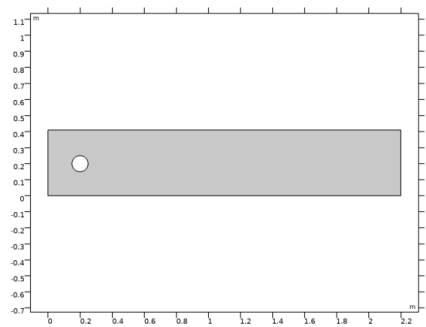
Select the object r1 only.
|
|
3
|
|
4
|
|
5
|
Select the object c1 only.
|
|
6
|
|
7
|
|
1
|
In the Model Builder window, under Component 1 (comp1) right-click Materials and choose Blank Material.
|
|
2
|
|
1
|
In the Model Builder window, under Component 1 (comp1) right-click Laminar Flow (spf) and choose Inlet.
|
|
3
|
|
4
|
|
1
|
|
1
|
|
2
|
|
3
|
|
4
|
|
1
|
|
2
|
|
3
|
|
1
|
|
2
|
|
3
|
|
4
|
|
5
|
|
1
|
|
2
|
In the Settings window for Particle Tracing with Mass, click to expand the Mass and Velocity section.
|
|
3
|
|
4
|
|
5
|
|
6
|
|
7
|
|
8
|
|
9
|
|
11
|
|
12
|
Click to expand the Coloring and Style section. Find the Line style subsection. From the Type list, choose None.
|
|
13
|
|
14
|
|
15
|
|
1
|
|
2
|
|
3
|
|
1
|
|
2
|
|
3
|
|
1
|
|
2
|
|
3
|
|
4
|
Select the Description check box.
|
|
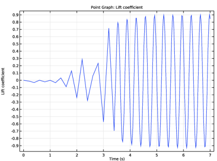
5
|
In the associated text field, type Lift coefficient.
|
|
6
|
|
1
|
|
2
|
|
3
|
|
1
|
|
2
|
|
3
|
|
4
|
Select the Description check box.
|
|
5
|
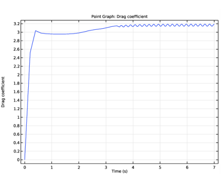
In the associated text field, type Drag coefficient.
|
|
6
|