PDF

Conical Quantum Dot
This application computes the electronic states for a quantum-dot/wetting-layer system. It was inspired largely by the work of Dr. M. Willatzen and Dr. R. Melnik (Ref. 1) as well as B. Lassen.
Introduction
Quantum dots are nanoscale or microscale devices created by confining free electrons in a 3D semiconducting matrix. The tiny islands or droplets of confined “free electrons” (those with no potential energy) present many interesting electronic properties. They are of potential importance for applications in quantum computing, biological labeling, and lasers, to name only a few.
Scientists can create such structures experimentally using the Stranski-Krastanow molecular beam-epitaxy technique. In that way they obtain 3D confinement regions (the quantum dots) by growth of a thin layer of material (the wetting layer) onto a semiconducting matrix. Quantum dots can have many geometries including cylindrical, conical, or pyramidal. This application studies the electronic states of a conical InAs quantum dot grown on a GaAs substrate.
To compute the electronic states taken on by the quantum dot/wetting layer assembly embedded in the GaAs surrounding matrix, you must solve the 1-band Schrödinger equation in the effective mass approximation:
where h is Planck’s constant, Ψ is the wave function, E is the eigenvalue (energy), and me is the effective electron mass (to account for screening effects).
Model Definition
The model works with the 1-particle stationary Schrödinger equation
It solves this eigenvalue problem for the quantum-dot/wetting-layer system using the following step potential barrier and effective-mass approximations:
V = 0 for the InAs quantum dot/wetting layer and V = 0.697 eV for the GaAs substrate.
me = 0.023m for InAs and me = 0.067m for GaAs.
Assume the quantum dot has perfect cylindrical symmetry. In that case you can model the overall structure in 2D as shown in the following figure.
Figure 1: 2D geometry of a perfectly cylindrical quantum dot and wetting layer.
You can now separate the total wave function Ψ into
where is the azimuthal angle. Then rewrite the Schrödinger equation in cylindrical coordinates as
Dividing this equation by
and rearranging its terms lead to the two independent equations
(1)
and
(2)
Equation 1 has obvious solutions of the form
where the periodicity condition implies that l, the principal quantum number, must be an integer. It remains to solve Equation 2, which you can rewrite as
Note that this is an instance of a PDE on coefficient form,
where the nonzero coefficients are
and λ = El.
Results
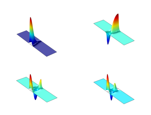
This exercise models the eigenvalues for the four lowest electronic energy levels for the principal quantum number  l = 0. The plots in Figure 2 show the eigenwave functions for those four states.
Figure 2: The four lowest electronic-energy levels for the case l = 0.
Notes About the COMSOL Implementation
To solve this problem, use the Coefficient Form PDE interface. The model solves for an eigenvalue/eigenfunction, for which you must input appropriate physical data and constants. Use electronvolts as the energy unit and nanometers as the length unit for the geometry.
Reference
1. R. Melnik and M. Willatzen, “Band structure of conical quantum dots with wetting layers,” Nanotechnology, vol. 15, pp. 1–8, 2004.
Application Library path: COMSOL_Multiphysics/Equation_Based/conical_quantum_dot
Modeling Instructions
From the File menu, choose New.
New
In the New window, click  Model Wizard.
Model Wizard
1
In the Model Wizard window, click  2D Axisymmetric.
2
In the Select Physics tree, select Mathematics>PDE Interfaces>Coefficient Form PDE (c).
3
Click Add.
4
Click  Study.
5
In the Select Study tree, select General Studies>Eigenvalue.
6
Global Definitions
Define dimensionless parameters for the electron mass and the reduced Planck constant expressed in electronvolt units. You can obtain these values by dividing the SI-unit values of the corresponding predefined COMSOL Multiphysics constants, me_const and hbar_const, by the value of the elementary charge e_const in coulombs.
Parameters 1
1
In the Model Builder window, under Global Definitions click Parameters 1.
2
In the Settings window for Parameters, locate the Parameters section.
3
Geometry 1
1
In the Model Builder window, under Component 1 (comp1) click Geometry 1.
2
In the Settings window for Geometry, locate the Units section.
3
From the Length unit list, choose nm.
Rectangle 1 (r1)
1
In the Geometry toolbar, click  Rectangle.
2
In the Settings window for Rectangle, locate the Size and Shape section.
3
In the Width text field, type 25.
4
In the Height text field, type 100.
5
Locate the Position section. From the Base list, choose Center.
6
In the r text field, type 12.5.
7
Click  Build Selected.
Rectangle 2 (r2)
1
In the Geometry toolbar, click  Rectangle.
2
In the Settings window for Rectangle, locate the Size and Shape section.
3
In the Width text field, type 25.
4
In the Height text field, type 2.
5
Locate the Position section. From the Base list, choose Center.
6
In the r text field, type 12.5.
7
Click  Build Selected.
Polygon 1 (pol1)
1
In the Geometry toolbar, click  Polygon.
2
In the Settings window for Polygon, locate the Coordinates section.
3
4
Click  Build Selected.
Compose 1 (co1)
1
In the Geometry toolbar, click  Booleans and Partitions and choose Compose.
2
Select the objects pol1 and r2 only.
3
In the Settings window for Compose, locate the Compose section.
4
In the Set formula text field, type r2+pol1.
5
Clear the Keep interior boundaries check box.
6
Click  Build Selected.
Compose 2 (co2)
1
In the Geometry toolbar, click  Booleans and Partitions and choose Compose.
2
Click in the Graphics window and then press Ctrl+A to select both objects.
3
In the Settings window for Compose, locate the Compose section.
4
In the Set formula text field, type r1+co1.
5
Click  Build Selected.
6
Click the  Zoom Extents button in the Graphics toolbar.
Coefficient Form PDE (c)
Coefficient Form PDE 1
1
In the Model Builder window, under Component 1 (comp1)>Coefficient Form PDE (c) click Coefficient Form PDE 1.
2
In the Settings window for Coefficient Form PDE, locate the Diffusion Coefficient section.
3
In the c text field, type c_In.
4
Locate the Absorption Coefficient section. In the a text field, type c_In*(l/r)^2+V_In.
5
Click to expand the Convection Coefficient section. Specify the β vector as
Coefficient Form PDE 2
1
In the Physics toolbar, click  Domains and choose Coefficient Form PDE.
2
3
In the Settings window for Coefficient Form PDE, locate the Diffusion Coefficient section.
4
In the c text field, type c_Ga.
5
Locate the Absorption Coefficient section. In the a text field, type c_Ga*(l/r)^2+V_Ga.
6
Click to expand the Convection Coefficient section. Specify the β vector as
Dirichlet Boundary Condition 1
1
In the Physics toolbar, click  Boundaries and choose Dirichlet Boundary Condition.
2
Mesh 1
In the Model Builder window, under Component 1 (comp1) right-click Mesh 1 and choose Build All.
Study 1
Step 1: Eigenvalue
1
In the Model Builder window, under Study 1 click Step 1: Eigenvalue.
2
In the Settings window for Eigenvalue, locate the Study Settings section.
3
Select the Desired number of eigenvalues check box.
4
5
In the Home toolbar, click  Compute.
Results
Follow the instructions below to reproduce the series of plots in Figure 2.
Height Expression 1
1
In the Model Builder window, expand the Results>2D Plot Group 1 node.
2
Right-click Surface 1 and choose Height Expression.
3
Click the  Zoom Extents button in the Graphics toolbar.
Compare the result to the upper-left plot in Figure 2.
2D Plot Group 1
1
In the Model Builder window, click 2D Plot Group 1.
2
In the Settings window for 2D Plot Group, locate the Data section.
3
From the Eigenvalue (rad/s) list, choose 0.39332.
4
In the 2D Plot Group 1 toolbar, click  Plot.
5
Click the  Zoom Extents button in the Graphics toolbar.
Compare the result to the upper-right plot in Figure 2.
6
From the Eigenvalue (rad/s) list, choose 0.4589.
7
In the 2D Plot Group 1 toolbar, click  Plot.
8
Click the  Zoom Extents button in the Graphics toolbar.
Compare the result to the lower-left plot in Figure 2.
9
From the Eigenvalue (rad/s) list, choose 0.56533.
10
In the 2D Plot Group 1 toolbar, click  Plot.
11
Click the  Zoom Extents button in the Graphics toolbar.
Compare the result to the lower-right plot in Figure 2.