PDF

Molecular Flow Through an RF Coupler
Introduction
Computing molecular flows in arbitrary geometries produces complex integral equations that are very difficult to compute analytically. There are two widely accepted methods for modeling molecular flows, the Monte Carlo method (which computes the trajectories of large numbers of randomized particles through the system) and the angular coefficient method. The Free Molecular Flow interfaces uses the angular coefficient method, which computes the molecular flow by summing the flux arriving at a surface from all other surfaces in its line of sight. The macroscopic variables in the vicinity of the surface can be derived from kinetic theory. The Mathematical Particle Tracing interface, available in the Particle Tracing Module can be used to implement the Monte Carlo method for molecular flows. The transmission probability can be computed and compared to the angular coefficient method.
Note: This application requires the Particle Tracing Module.
Model Definition
Particle trajectories are computed using Newton’s law of motion:
The particle velocity is given by:
When the particles encounter a boundary, they scatter according to Knudsen’s law.
where the subscript t denotes the tangential component of the velocity and n the normal. In addition, c is the particle speed which is sampled from the following probability density function:
This is accomplished using the normally distributed random function, which is used to assign a new normally distributed random speed to each particle at each time step. The angle φ is a uniformly distributed random number between 0 and π. The angle, θ is a random angle, which is defined by the piecewise function:
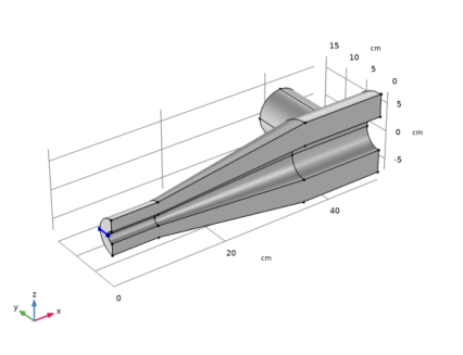
where g is a random number between 0 and 1. In all 10,000 particles are released into the modeling domain. The number of particles that reaches the outlet boundary determines the transmission probability.
The transmission probability for the molecular flow interface is given by the following:
Results and Discussion
The molecular flux computed by the angular coefficient method is shown in Figure 1. The transmission probability based on this is computed to be 0.21749. Using the particle based approach the transmission probability comes out to be 0.2136. Of course, using stricter tolerances and including more particles in the simulation provides better agreement with the angular coefficient method, at the expense of additional CPU time.
Figure 1: Plot of the incident molecular flux.
Notes About the COMSOL Implementation
The model is solved in two stages. First the Free Molecular Flow interface is used to compute the transmission probability using a Stationary study. Subsequently, the Mathematical Particle Tracing interface is used to compute the transmission probability with a Time Dependent study using a Monte Carlo approach.
Application Library path: Molecular_Flow_Module/Benchmarks/rf_coupler
Modeling Instructions
From the File menu, choose New.
New
In the New window, click  Model Wizard.
Model Wizard
1
In the Model Wizard window, click  3D.
2
In the Select Physics tree, select Fluid Flow>Rarefied Flow>Free Molecular Flow (fmf).
3
Click Add.
4
Click  Study.
5
In the Select Study tree, select General Studies>Stationary.
6
Global Definitions
Parameters 1
1
In the Model Builder window, under Global Definitions click Parameters 1.
2
In the Settings window for Parameters, locate the Parameters section.
3
Geometry 1
1
In the Model Builder window, under Component 1 (comp1) click Geometry 1.
2
In the Settings window for Geometry, locate the Units section.
3
From the Length unit list, choose cm.
Use a work plane to define the model geometry.
Work Plane 1 (wp1)
1
In the Geometry toolbar, click  Work Plane.
2
In the Settings window for Work Plane, locate the Plane Definition section.
3
From the Plane list, choose yx-plane.
4
Click  Show Work Plane.
Work Plane 1 (wp1)>Rectangle 1 (r1)
1
In the Work Plane toolbar, click  Rectangle.
2
In the Settings window for Rectangle, locate the Size and Shape section.
3
In the Width text field, type 2.
4
In the Height text field, type 8.
5
Locate the Position section. In the xw text field, type 1.
6
In the Work Plane toolbar, click  Build All.
Work Plane 1 (wp1)>Polygon 1 (pol1)
1
In the Work Plane toolbar, click  Polygon.
2
In the Settings window for Polygon, locate the Coordinates section.
3
From the Data source list, choose Vectors.
4
In the xw text field, type 1 3 3 7 7 3 3 1.
5
In the yw text field, type 8 35 35 35 35 8 8 8.
6
In the Work Plane toolbar, click  Build All.
7
Click the  Zoom Extents button in the Graphics toolbar.
Work Plane 1 (wp1)>Rectangle 2 (r2)
1
In the Work Plane toolbar, click  Rectangle.
2
In the Settings window for Rectangle, locate the Size and Shape section.
3
In the Width text field, type 4.
4
In the Height text field, type 15.
5
Locate the Position section. In the xw text field, type 3.
6
In the yw text field, type 35.
Work Plane 1 (wp1)>Union 1 (uni1)
1
In the Work Plane toolbar, click  Booleans and Partitions and choose Union.
2
Click in the Graphics window and then press Ctrl+A to select all objects.
3
In the Settings window for Union, locate the Union section.
4
Clear the Keep interior boundaries check box.
5
In the Work Plane toolbar, click  Build All.
6
Click the  Zoom Extents button in the Graphics toolbar.
Revolve 1 (rev1)
1
In the Model Builder window, right-click Geometry 1 and choose Revolve.
2
In the Settings window for Revolve, locate the Revolution Angles section.
3
Click the Angles button.
4
In the Start angle text field, type -90.
5
In the End angle text field, type 90.
6
Click  Build All Objects.
7
Click the  Go to Default View button in the Graphics toolbar.
Cylinder 1 (cyl1)
1
In the Geometry toolbar, click  Cylinder.
2
In the Settings window for Cylinder, locate the Size and Shape section.
3
In the Radius text field, type 4.
4
In the Height text field, type 10.
5
Locate the Position section. In the x text field, type 42.
6
In the y text field, type 5.
7
Locate the Axis section. From the Axis type list, choose y-axis.
8
Click  Build All Objects.
Union 1 (uni1)
1
In the Geometry toolbar, click  Booleans and Partitions and choose Union.
2
Click in the Graphics window and then press Ctrl+A to select both objects.
3
In the Settings window for Union, locate the Union section.
4
Clear the Keep interior boundaries check box.
5
Click  Build All Objects.
Ignore Edges 1 (ige1)
1
In the Geometry toolbar, click  Virtual Operations and choose Ignore Edges.
2
On the object fin, select Edge 11 only.
It might be easier to select the correct edge by using the Selection List window. To open this window, in the Home toolbar click Windows and choose Selection List. (If you are running the cross-platform desktop, you find Windows in the main menu.)
Free Molecular Flow (fmf)
Molecular Flow 1
1
In the Model Builder window, under Component 1 (comp1)>Free Molecular Flow (fmf) click Molecular Flow 1.
2
In the Settings window for Molecular Flow, locate the Molecular Weight of Species section.
3
In the Mn,G text field, type Mw.
Surface Temperature 1
1
In the Model Builder window, click Surface Temperature 1.
2
In the Settings window for Surface Temperature, locate the Surface Temperature section.
3
In the T text field, type T0.
Reservoir 1
1
In the Physics toolbar, click  Boundaries and choose Reservoir.
2
3
In the Settings window for Reservoir, locate the Reservoir section.
4
In the p0,G text field, type p0.
Vacuum Pump 1
1
In the Physics toolbar, click  Boundaries and choose Vacuum Pump.
2
Click the  Wireframe Rendering button in the Graphics toolbar.
3
4
In the Settings window for Vacuum Pump, locate the Vacuum Pump section.
5
In the fG text field, type frac.
Free Molecular Flow (fmf)
Plane Symmetry 1
1
In the Model Builder window, expand the Component 1 (comp1)>Definitions node.
2
Right-click Component 1 (comp1)>Free Molecular Flow (fmf) and choose Plane Symmetry.
3
Definitions
Define a nonlocal integration coupling on the inlet and outlet to help compute the transmission probability.
Integration 1 (intop1)
1
In the Definitions toolbar, click  Nonlocal Couplings and choose Integration.
2
In the Settings window for Integration, locate the Source Selection section.
3
From the Geometric entity level list, choose Boundary.
4
Integration 2 (intop2)
1
In the Definitions toolbar, click  Nonlocal Couplings and choose Integration.
2
In the Settings window for Integration, locate the Source Selection section.
3
From the Geometric entity level list, choose Boundary.
4
Molecular Flow Variables
1
In the Definitions toolbar, click  Local Variables.
2
Right-click Variables 1 and choose Rename.
3
In the Rename Variables dialog box, type Molecular Flow Variables in the New label text field.
4
5
In the Settings window for Variables, locate the Variables section.
6
Mesh 1
1
In the Settings window for Mesh, locate the Physics-Controlled Mesh section.
2
From the Element size list, choose Finer.
3
Click  Build All.
Study 1
In the Home toolbar, click  Compute.
Results
Mirror 3D 1
1
In the Results toolbar, click  More Datasets and choose Mirror 3D.
2
In the Settings window for Mirror 3D, locate the Plane Data section.
3
From the Plane list, choose ZX-planes.
Now add a Mirror 3D dataset to visualize the entire geometry in results.
Incident Molecular Flux (fmf)
1
In the Model Builder window, click Incident Molecular Flux (fmf).
2
In the Settings window for 3D Plot Group, locate the Data section.
3
From the Dataset list, choose Mirror 3D 1.
4
In the Incident Molecular Flux (fmf) toolbar, click  Plot.
Now evaluate the transmission probability.
Global Evaluation 1
1
In the Results toolbar, click  Global Evaluation.
2
In the Settings window for Global Evaluation, click Replace Expression in the upper-right corner of the Expressions section. From the menu, choose Component 1 (comp1)>Definitions>Variables>alpha - Transmission probability.
3
Click  Evaluate.
Component 1 (comp1)
Now add the mathematical particle tracing interface to compute the transmission probability with a Monte Carlo approach.
Add Physics
1
In the Home toolbar, click  Add Physics to open the Add Physics window.
2
Go to the Add Physics window.
3
In the tree, select Mathematics>Mathematical Particle Tracing (pt).
4
Find the Physics interfaces in study subsection. In the table, clear the Solve check box for Study 1.
5
Click Add to Component 1 in the window toolbar.
6
In the Home toolbar, click  Add Physics to close the Add Physics window.
Add Study
1
In the Home toolbar, click  Add Study to open the Add Study window.
2
Go to the Add Study window.
3
Find the Studies subsection. In the Select Study tree, select General Studies>Time Dependent.
4
Find the Physics interfaces in study subsection. In the table, clear the Solve check box for Free Molecular Flow (fmf).
5
Click Add Study in the window toolbar.
6
In the Home toolbar, click  Add Study to close the Add Study window.
Mathematical Particle Tracing (pt)
1
In the Model Builder window, under Component 1 (comp1) click Mathematical Particle Tracing (pt).
2
In the Settings window for Mathematical Particle Tracing, locate the Particle Release and Propagation section.
3
In the Maximum number of secondary particles text field, type 0.
Global Definitions
Parameters 1
1
In the Model Builder window, under Global Definitions click Parameters 1.
2
In the Settings window for Parameters, locate the Parameters section.
3
Mathematical Particle Tracing (pt)
Particle Properties 1
1
In the Model Builder window, under Component 1 (comp1)>Mathematical Particle Tracing (pt) click Particle Properties 1.
2
In the Settings window for Particle Properties, locate the Particle Mass section.
3
In the mp text field, type M.
Inlet 1
1
In the Physics toolbar, click  Boundaries and choose Inlet.
2
Release 10,000 particles uniformly spaced over the inlet boundary. Use the Thermal initial velocity to release the particles.
3
In the Settings window for Inlet, locate the Initial Position section.
4
From the Initial position list, choose Projected plane grid.
5
In the N text field, type 10000.
6
Locate the Initial Velocity section. From the Initial velocity list, choose Thermal.
7
In the T text field, type T0.
Thermal Re-Emission 1
1
In the Physics toolbar, click  Boundaries and choose Thermal Re-Emission.
2
In the Settings window for Thermal Re-Emission, locate the Boundary Selection section.
3
From the Selection list, choose All boundaries.
4
Locate the Wall Properties section. In the T text field, type T0.
Thermal Re-Emission 2
1
In the Physics toolbar, click  Boundaries and choose Thermal Re-Emission.
2
3
In the Settings window for Thermal Re-Emission, locate the Wall Properties section.
4
In the T text field, type T0.
5
In the γ text field, type frac.
Particle Counter 1
1
In the Physics toolbar, click  Boundaries and choose Particle Counter.
2
3
In the Settings window for Particle Counter, locate the Particle Counter section.
4
From the Release feature list, choose Inlet 1.
Create a Wall boundary condition to contribute with the inlet boundary. This ensures that particles returning to the inlet will disappear.
Wall 2
1
In the Physics toolbar, click  Boundaries and choose Wall.
2
3
In the Settings window for Wall, locate the Wall Condition section.
4
From the Wall condition list, choose Disappear.
Create a bounce Wall boundary condition to provide a symmetry condition.
Wall 3
1
In the Physics toolbar, click  Boundaries and choose Wall.
2
3
In the Settings window for Wall, locate the Wall Condition section.
4
From the Wall condition list, choose Bounce.
Component 1 (comp1)
In order to obtain an accurate solution, a very fine mesh should be used. Since the only degrees of freedom correspond to the particles, using a very fine mesh does not significantly add to the computational burden.
Mesh 2
1
In the Mesh toolbar, click  Add Mesh.
2
In the Settings window for Mesh, locate the Physics-Controlled Mesh section.
3
From the Element size list, choose Extremely fine.
4
Click  Build All.
The solver settings for the particle tracing need to be quite strict in order to obtain an accurate transmission probability. The initial timestep should be very small in comparison to the total simulation time and the maximum time step should be small enough to accurately resolve the particle trajectories.
Study 2
Step 1: Time Dependent
1
In the Model Builder window, under Study 2 click Step 1: Time Dependent.
2
In the Settings window for Time Dependent, locate the Study Settings section.
3
In the Output times text field, type range(0,0.03/49,0.03).
4
Click to expand the Mesh Selection section. In the table, enter the following settings:
Solution 2 (sol2)
1
In the Study toolbar, click  Show Default Solver.
2
In the Model Builder window, expand the Solution 2 (sol2) node, then click Time-Dependent Solver 1.
3
In the Settings window for Time-Dependent Solver, click to expand the Time Stepping section.
4
Select the Initial step check box.
5
6
From the Maximum step constraint list, choose Constant.
7
In the Maximum step text field, type 1e-4.
8
In the Study toolbar, click  Compute.
Results
Particle Trajectories (pt)
After the study is complete, a Warning node may appear in the solver sequence, indicating that some particles have been removed from the simulation because an intersection point with the boundary was not found. This occasionally happens because of the discretization of the chamber walls using the finite element mesh, which is an imperfect representation of cylindrical and conical boundaries. Usually the number of removed particles is very small compared to the total number of particles and can safely be ignored.
If it is absolutely necessary to prevent any particles from disappearing in this manner, you can reduce the probability of rays failing to detect boundary intersections by further refining the mesh. Also consider selecting Linear from the Geometry shape order list in the Component 1 settings; linear shape order is more robust than the default shape order, which is mostly quadratic, at the expense of some accuracy.
Global Evaluation 2
1
In the Results toolbar, click  Global Evaluation.
2
In the Settings window for Global Evaluation, locate the Data section.
3
From the Dataset list, choose Study 2/Solution 2 (sol2).
4
From the Time selection list, choose Last.
5
Click Replace Expression in the upper-right corner of the Expressions section. From the menu, choose Component 1 (comp1)>Mathematical Particle Tracing>Particle Counter 1>pt.pcnt1.alpha - Transmission probability.
The transmission probability from the particle tracing approach agrees very well with the result from the Free Molecular Flow interface.
6
Click  Evaluate.