PDF

Molecular Flow in an Ion-Implant Vacuum System
Introduction
This example considers the design of an ion implantation system. Ion implantation is used extensively in the semiconductor industry to implant dopants into wafers. Within an ion implanter ions generated within an ion source are accelerated by an electric field to achieve the desired implant energy. Ions of the correct charge state are selected by means of a separation magnet which bends the ion beam to ensure that ions of a particular charge to mass ratio are the only ones which reach the wafer. The energy dose and angle of the ion beam are both key parameters for the process. This part of the system is known as the corrector.
Usually it is desired that only selected regions of the wafer are implanted. This is achieved by masking parts of the wafer with an organic photoresist, to produce the desired pattern. Unfortunately, the photoresist itself emits gas molecules as a result of the beam striking it. These molecules can interact with the ion beam and produce species with undesired charge to mass ratios at different points along the beam path. Some of these species may reach the wafer, degrading the uniformity of the implant, which is highly undesirable. Additionally, these ions may also effect the accuracy of measurements of the implant dose. A key requirement for the system is that the number density of the outgassing molecules for the wafer is low within the beam line.
This example shows how to model an ion implantation system using the Molecular Flow interface. Because it is interactions of outgassing molecules with the beam that produce undesirable species, the average number density of these molecules along the beam path is used as a figure of merit to evaluate the design. Furthermore, because the angle of the wafer to the beam can be modified, the figure of merit must be computed as a function of wafer angle, with rotation about one axis.
Figure 1: Model geometry. Key components of the system are labeled. The red line through the center of the wafer carrier indicates the axis of rotation of the carrier.
Note: This model is motivated by Ref. 1. However, it is important to note that there are significant differences between the pressure and number density computed by the Molecular Flow interface and those computed in the radiation analogy, which is used in Ref. 1. The COMSOL Multiphysics software computes these quantities accurately, whilst the radiation analogy uses an approximate technique to compute the number density and pressure which can result in misleading, incorrect, answers.
Model Definition
The model geometry is shown in Figure 1. The wafer is positioned on a carrier plate which is rotated about an axis through its center to achieve different implant angles. The carrier plate is mounted in a chamber that is pumped by three large cryopumps, on cylindrical vacuum ports. These pumps have a pump speed of 12,000 l/s. In this model outgassing of only one species from the wafer (H2) is considered: multiple species can be modeled by adding additional molecular flow interfaces. It is assumed that the outgassing across the wafer surface is uniform and that the total gas emitted is 30 sccm. The vacuum path through the corrector magnetic field enters the main chamber opposite the wafer, and is pumped by a turbomolecular pump on a cylindrical port midway down the corrector, with a pump speed of 1500 l/s and an additional cryopump at the start of the beam path, with a pump speed of 12,000 l/s. There is an aperture at the entrance to the chamber which reduces the flux that enters the corrector. The angle of the wafer normal to the ion beam is swept from 0° to 60° in 20° steps, as the wafer is rotated about the horizontal axis through its center, as shown in Figure 1. All other surfaces in the model are walls.
Results and Discussion
The molecular flux at the surfaces of the vacuum chamber is shown in Figure 2, for wafer normal angles of 0° and 40° to the beam.
The shadowing effect of the wafer support is evident at both wafer angles shown in Figure 2. It is also clear that more flux enters the beam line when the wafer normal is parallel to the beam because the line of sight with the beam line is then parallel to the wafer normal. The number density along the beam path is shown in Figure 3 for each of the angles solved for. The number density increases along the beam path toward the wafer, with strong changes in gradient as the beam passes through different apertures. Note that in the immediate vicinity of the wafer the number density is not computed accurately (this is difficult to see from the plot below, but zooming into the plot at the end of the beam shows issues in the results for elements adjacent to the surface). This is a result of numerical issues when computing the number density very close to a source surface within the domain.
The average number density along the beam path within the corrector can be used as figure of merit for the system design. This quantity is plotted against the angle of the wafer normal to the beam line in Figure 4. The average flux in the corrector is reduced by rotating the wafer normal away from the beam line with a 10% reduction occurring over the full angular range. Rotating the wafer in this manner can therefore result in improved performance of the implanter.
Figure 2: Pressure on the surface of the ion implanter, with the wafer normal at 0° (top) and 40° (bottom) to the beam path.
Figure 3: The number density as a function of position along the beam line.
Figure 4: Plot of the average number density along the beam line as a function of the wafer normal angle to the incoming beam.
Reference
1. M.R. LaFontaine, N. Tokoro, P. Murphy, and D. Holbrook, “Modelling Photoresist Outgassing Pressure Distribution Using the Finite Element Method,” Proc. Conference on Ion Implantation Technology, IEEE Press, pp. 247–250, 2000.
Notes About the COMSOL Implementation
The model is straightforward to set up using the Molecular Flow interface. The vacuum pump boundary condition is used for the pumps and the outgassing wall boundary condition is used for the wafer surface. The geometry for the vacuum system is imported, but the wafer and its carrier are generated within COMSOL Multiphysics so that the angle to the beam line can be easily parameterized.
Application Library path: Molecular_Flow_Module/Industrial_Applications/ion_implanter
Modeling Instructions
From the File menu, choose New.
New
In the New window, click  Model Wizard.
Model Wizard
1
In the Model Wizard window, click  3D.
2
In the Select Physics tree, select Fluid Flow>Rarefied Flow>Free Molecular Flow (fmf).
3
Click Add.
4
Click  Study.
5
In the Select Study tree, select General Studies>Stationary.
6
Set up parameters for the wafer angle and pump speeds.
Global Definitions
Parameters 1
1
In the Model Builder window, under Global Definitions click Parameters 1.
2
In the Settings window for Parameters, locate the Parameters section.
3
For convenience, the device geometry is inserted from an existing file. You can read the instructions for creating the geometry in the Appendix - Geometry Instructions.
Geometry 1
1
In the Geometry toolbar, click  Insert Sequence.
2
3
In the Geometry toolbar, click  Build All.
Add a nonlocal average coupling to compute the average number density along the beam line.
Definitions
Beam line
1
In the Definitions toolbar, click  Explicit.
2
In the Settings window for Explicit, locate the Input Entities section.
3
From the Geometric entity level list, choose Edge.
4
5
In the Label text field, type Beam line.
Average 1 (aveop1)
1
In the Definitions toolbar, click  Nonlocal Couplings and choose Average.
2
In the Settings window for Average, locate the Source Selection section.
3
From the Geometric entity level list, choose Edge.
4
Click the  Wireframe Rendering button in the Graphics toolbar.
5
From the Selection list, choose Beam line.
Set the physics interface to simulate free molecular flow of hydrogen.
Free Molecular Flow (fmf)
Molecular Flow 1
1
In the Model Builder window, under Component 1 (comp1)>Free Molecular Flow (fmf) click Molecular Flow 1.
2
In the Settings window for Molecular Flow, locate the Molecular Weight of Species section.
3
In the Mn,G text field, type 0.002[kg/mol].
Set up the wafer to outgass 30 sccm of hydrogen.
Wall 2
1
In the Physics toolbar, click  Boundaries and choose Wall.
2
3
In the Settings window for Wall, locate the Wall Type section.
4
From the Wall type list, choose Outgassing wall.
5
Locate the Flux section. From the Outgoing flux list, choose Number of SCCM units.
6
In the Qsccm,G text field, type 30.
Set up the vacuum pumps.
Vacuum Pump 1
1
In the Physics toolbar, click  Boundaries and choose Vacuum Pump.
2
In the Settings window for Vacuum Pump, locate the Vacuum Pump section.
3
From the Specify pump flux list, choose Pump speed.
4
5
In the SG text field, type pumpspeedturbo.
Vacuum Pump 2
1
In the Physics toolbar, click  Boundaries and choose Vacuum Pump.
2
In the Settings window for Vacuum Pump, locate the Vacuum Pump section.
3
From the Specify pump flux list, choose Pump speed.
4
5
In the SG text field, type pumpspeedcryo.
Vacuum Pump 3
1
Right-click Vacuum Pump 2 and choose Duplicate.
2
In the Settings window for Vacuum Pump, locate the Boundary Selection section.
3
Click  Clear Selection.
4
Vacuum Pump 4
1
Right-click Vacuum Pump 3 and choose Duplicate.
2
In the Settings window for Vacuum Pump, locate the Boundary Selection section.
3
Click  Clear Selection.
4
Vacuum Pump 5
1
Right-click Vacuum Pump 4 and choose Duplicate.
2
In the Settings window for Vacuum Pump, locate the Boundary Selection section.
3
Click  Clear Selection.
4
Number Density Reconstruction 1
1
In the Physics toolbar, click  Edges and choose Number Density Reconstruction.
2
In the Settings window for Number Density Reconstruction, locate the Edge Selection section.
3
From the Selection list, choose Beam line.
Next create the mesh. Add a fine mesh along the beam line.
Mesh 1
Edge 1
1
In the Mesh toolbar, click  Boundary and choose Edge.
2
In the Settings window for Edge, locate the Edge Selection section.
3
From the Selection list, choose Beam line.
Use a very fine mesh along the beam line.
Size 1
1
Right-click Edge 1 and choose Size.
2
In the Settings window for Size, locate the Element Size section.
3
Click the Custom button.
4
Locate the Element Size Parameters section. Select the Maximum element size check box.
5
Change the global mesh size setting to refine the mesh.
Size
1
In the Model Builder window, click Size.
2
In the Settings window for Size, locate the Element Size section.
3
From the Predefined list, choose Extra fine.
Add a free triangular surface mesh. This will inherit the global mesh size setting.
Free Triangular 1
1
In the Mesh toolbar, click  Boundary and choose Free Triangular.
2
In the Settings window for Free Triangular, locate the Boundary Selection section.
3
From the Selection list, choose All boundaries.
4
Click  Build All.
The domain does not need to be meshed since the interface solves equations only on the surfaces of the model. Note that it is possible to mesh surfaces edges and points (as in this model) or to mesh the entire domain. These two approaches cannot be mixed (doing so may lead to incorrect results in some cases).
Set up a parametric sweep over the wafer angle. The study will take approximately 4 minutes to complete with the full sweep. Alternatively it is possible to solve for a single wafer angle to save time.
Study 1
Parametric Sweep
1
In the Study toolbar, click  Parametric Sweep.
2
In the Settings window for Parametric Sweep, locate the Study Settings section.
3
4
5
Click  Range.
6
In the Range dialog box, type 0 in the Start text field.
7
In the Step text field, type 20.
8
In the Stop text field, type 60.
9
Click Add.
10
In the Study toolbar, click  Compute.
Results
Incident Molecular Flux (fmf)
Create a duplicate solution with a selection so that you can see inside the vacuum chamber.
Study 1/Parametric Solutions 1 (3) (sol2)
1
In the Model Builder window, expand the Results>Datasets node.
2
Right-click Results>Datasets>Study 1/Parametric Solutions 1 (sol2) and choose Duplicate.
Selection
1
In the Results toolbar, click  Attributes and choose Selection.
2
In the Settings window for Selection, locate the Geometric Entity Selection section.
3
From the Geometric entity level list, choose Boundary.
4
From the Selection list, choose Postprocessing.
Update the default plots to use the new dataset.
Incident Molecular Flux (fmf)
1
In the Model Builder window, click Incident Molecular Flux (fmf).
2
In the Settings window for 3D Plot Group, locate the Data section.
3
From the Dataset list, choose Study 1/Parametric Solutions 1 (3) (sol2).
Total Number Density (fmf)
1
In the Model Builder window, click Total Number Density (fmf).
2
In the Settings window for 3D Plot Group, locate the Data section.
3
From the Dataset list, choose Study 1/Parametric Solutions 1 (3) (sol2).
Total Pressure (fmf)
1
In the Model Builder window, click Total Pressure (fmf).
2
In the Settings window for 3D Plot Group, locate the Data section.
3
From the Dataset list, choose Study 1/Parametric Solutions 1 (3) (sol2).
Reproduce the results shown in Figure 2.
Total Number Density (fmf)
1
In the Model Builder window, click Total Number Density (fmf).
2
In the Settings window for 3D Plot Group, locate the Data section.
3
From the Parameter value (theta (deg)) list, choose 0.
4
In the Total Number Density (fmf) toolbar, click  Plot.
Repeat steps 3 and 4, this time selecting an angle of 40 degrees.
Compare the resulting plot with that in Figure 2.
Create a plot of the number density along the beam path.
Number Density Along Beam Line
1
In the Home toolbar, click  Add Plot Group and choose 1D Plot Group.
2
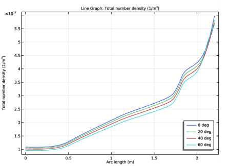
In the Settings window for 1D Plot Group, type Number Density Along Beam Line in the Label text field.
3
Locate the Data section. From the Dataset list, choose Study 1/Parametric Solutions 1 (2) (sol2).
4
Locate the Legend section. From the Position list, choose Lower right.
Line Graph 1
1
Right-click Number Density Along Beam Line and choose Line Graph.
2
In the Settings window for Line Graph, locate the Selection section.
3
From the Selection list, choose Beam line.
4
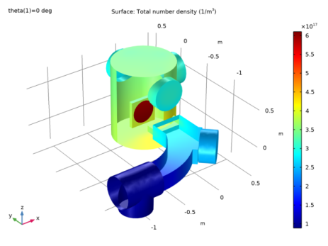
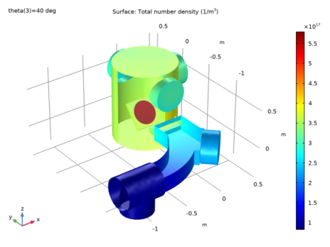
Click Replace Expression in the upper-right corner of the y-Axis Data section. From the menu, choose Component 1 (comp1)>Free Molecular Flow>Number density>fmf.ntot - Total number density - 1/m³.
5
Click to expand the Legends section. Select the Show legends check box.
6
Click to expand the Quality section. From the Resolution list, choose No refinement.
7
In the Number Density Along Beam Line toolbar, click  Plot.
Compare the resulting plot with that in Figure 3.
Finally, plot the mean number density along the beam line, as a function of wafer angle.
Average Number Density vs. Wafer Angle
1
In the Home toolbar, click  Add Plot Group and choose 1D Plot Group.
2
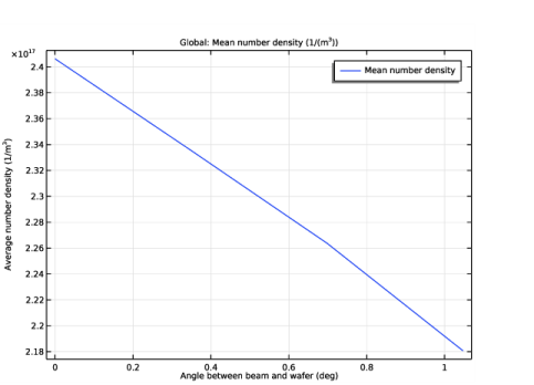
In the Settings window for 1D Plot Group, type Average Number Density vs. Wafer Angle in the Label text field.
3
Locate the Data section. From the Dataset list, choose Study 1/Parametric Solutions 1 (2) (sol2).
4
Locate the Plot Settings section. Select the x-axis label check box.
5
In the associated text field, type Angle between beam and wafer (deg).
6
Select the y-axis label check box.
7
In the associated text field, type Average number density (1/m<sup>3</sup>).
Global 1
1
Right-click Average Number Density vs. Wafer Angle and choose Global.
2
In the Settings window for Global, locate the y-Axis Data section.
3
4
Locate the x-Axis Data section. From the Parameter list, choose Expression.
5
In the Expression text field, type theta.
6
In the Average Number Density vs. Wafer Angle toolbar, click  Plot.
Compare the resulting plot with that in Figure 4.
Appendix - Geometry Instructions
From the File menu, choose New.
New
In the New window, click  Blank Model.
Global Definitions
Parameters 1
1
In the Model Builder window, under Global Definitions click Parameters 1.
2
In the Settings window for Parameters, locate the Parameters section.
3
Add Component
In the Home toolbar, click  Add Component and choose 3D.
Geometry 1
Cylinder 1 (cyl1)
1
In the Geometry toolbar, click  Cylinder.
2
In the Settings window for Cylinder, locate the Size and Shape section.
3
In the Radius text field, type 0.4.
4
Locate the Position section. In the z text field, type -0.3.
Cylinder 2 (cyl2)
1
In the Geometry toolbar, click  Cylinder.
2
In the Settings window for Cylinder, locate the Size and Shape section.
3
In the Radius text field, type 0.2.
4
In the Height text field, type 0.5.
5
Locate the Position section. In the y text field, type -0.5.
6
In the z text field, type 0.45.
7
Locate the Axis section. From the Axis type list, choose y-axis.
Rotate 1 (rot1)
1
In the Geometry toolbar, click  Transforms and choose Rotate.
2
3
In the Settings window for Rotate, locate the Rotation section.
4
In the Angle text field, type 0,90,180.
Cylinder 3 (cyl3)
1
In the Geometry toolbar, click  Cylinder.
2
In the Settings window for Cylinder, locate the Size and Shape section.
3
In the Radius text field, type 0.2.
4
In the Height text field, type 0.5.
5
Locate the Position section. In the x text field, type -1.3.
6
In the y text field, type -1.25.
7
Locate the Axis section. From the Axis type list, choose x-axis.
Cylinder 4 (cyl4)
1
In the Geometry toolbar, click  Cylinder.
2
In the Settings window for Cylinder, locate the Size and Shape section.
3
In the Radius text field, type 0.2.
4
In the Height text field, type 0.3.
5
Locate the Position section. In the x text field, type -1.05.
6
In the y text field, type -1.25.
7
In the z text field, type -0.3.
Block 1 (blk1)
1
In the Geometry toolbar, click  Block.
2
In the Settings window for Block, locate the Size and Shape section.
3
In the Width text field, type 0.4.
4
In the Depth text field, type 0.2.
5
In the Height text field, type 0.08.
6
Locate the Position section. In the x text field, type -0.2.
7
In the y text field, type -0.45.
8
In the z text field, type -0.04.
Work Plane 1 (wp1)
1
In the Geometry toolbar, click  Work Plane.
2
In the Settings window for Work Plane, locate the Selections of Resulting Entities section.
3
Select the Resulting objects selection check box.
4
From the Show in physics list, choose All levels.
Work Plane 1 (wp1)>Plane Geometry
In the Model Builder window, click Plane Geometry.
Work Plane 1 (wp1)>Circle 1 (c1)
1
In the Work Plane toolbar, click  Circle.
2
In the Settings window for Circle, locate the Size and Shape section.
3
In the Radius text field, type 0.8.
4
In the Sector angle text field, type 90.
5
Locate the Position section. In the xw text field, type -0.8.
6
In the yw text field, type -0.45.
7
Locate the Rotation Angle section. In the Rotation text field, type -90.
8
Locate the Object Type section. From the Type list, choose Curve.
Work Plane 1 (wp1)>Rectangle 1 (r1)
1
In the Work Plane toolbar, click  Rectangle.
2
In the Settings window for Rectangle, locate the Object Type section.
3
From the Type list, choose Curve.
4
Locate the Size and Shape section. In the Width text field, type 1.3.
5
In the Height text field, type 1.25.
6
Locate the Position section. In the xw text field, type -1.3.
7
In the yw text field, type -1.25.
Work Plane 1 (wp1)>Union 1 (uni1)
1
In the Work Plane toolbar, click  Booleans and Partitions and choose Union.
2
Click in the Graphics window and then press Ctrl+A to select both objects.
3
In the Settings window for Union, click  Build Selected.
Work Plane 1 (wp1)>Delete Entities 1 (del1)
1
In the Work Plane toolbar, click  Delete.
2
In the Settings window for Delete Entities, locate the Entities or Objects to Delete section.
3
From the Geometric entity level list, choose Boundary.
4
On the object uni1, select Boundaries 1 and 3–7 only.
Work Plane 2 (wp2)
1
In the Model Builder window, under Component 1 (comp1)>Geometry 1 right-click Work Plane 1 (wp1) and choose Work Plane.
2
In the Settings window for Work Plane, locate the Plane Definition section.
3
In the z-coordinate text field, type 0.1.
Work Plane 2 (wp2)>Plane Geometry
In the Model Builder window, click Plane Geometry.
Work Plane 2 (wp2)>Circle 1 (c1)
1
In the Work Plane toolbar, click  Circle.
2
In the Settings window for Circle, locate the Object Type section.
3
From the Type list, choose Curve.
4
Locate the Size and Shape section. In the Radius text field, type 0.95.
5
In the Sector angle text field, type 90.
6
Locate the Position section. In the xw text field, type -0.8.
7
In the yw text field, type -0.45.
8
Locate the Rotation Angle section. In the Rotation text field, type -90.
9
Click to expand the Layers section. In the table, enter the following settings:
10
Click  Build Selected.
Work Plane 2 (wp2)>Delete Entities 1 (del1)
1
In the Work Plane toolbar, click  Delete.
2
In the Settings window for Delete Entities, locate the Entities or Objects to Delete section.
3
From the Geometric entity level list, choose Boundary.
4
On the object c1, select Boundaries 1 and 2 only.
Work Plane 2 (wp2)>Rectangle 1 (r1)
1
In the Work Plane toolbar, click  Rectangle.
2
In the Settings window for Rectangle, locate the Size and Shape section.
3
In the Width text field, type 0.4.
4
In the Height text field, type 0.36.
5
Locate the Position section. In the xw text field, type -0.2.
6
In the yw text field, type -0.81.
Work Plane 2 (wp2)>Rectangle 2 (r2)
1
In the Work Plane toolbar, click  Rectangle.
2
In the Settings window for Rectangle, locate the Size and Shape section.
3
In the Width text field, type 0.5.
4
In the Height text field, type 0.25.
5
Locate the Position section. In the xw text field, type -0.12.
6
In the yw text field, type -1.2.
7
Locate the Rotation Angle section. In the Rotation text field, type 45.
Work Plane 2 (wp2)>Union 1 (uni1)
1
In the Work Plane toolbar, click  Booleans and Partitions and choose Union.
2
Click in the Graphics window and then press Ctrl+A to select all objects.
3
In the Settings window for Union, locate the Union section.
4
Clear the Keep interior boundaries check box.
Extrude 1 (ext1)
1
In the Model Builder window, under Component 1 (comp1)>Geometry 1 right-click Work Plane 2 (wp2) and choose Extrude.
2
In the Settings window for Extrude, locate the Distances section.
3
4
Select the Reverse direction check box.
Work Plane 3 (wp3)
1
In the Geometry toolbar, click  Work Plane.
2
In the Settings window for Work Plane, locate the Plane Definition section.
3
From the Plane type list, choose Face parallel.
4
On the object ext1, select Boundary 10 only.
Work Plane 3 (wp3)>Plane Geometry
In the Model Builder window, click Plane Geometry.
Work Plane 3 (wp3)>Circle 1 (c1)
1
In the Work Plane toolbar, click  Circle.
2
In the Settings window for Circle, locate the Size and Shape section.
3
In the Radius text field, type 0.2.
Extrude 2 (ext2)
1
In the Model Builder window, under Component 1 (comp1)>Geometry 1 right-click Work Plane 3 (wp3) and choose Extrude.
2
In the Settings window for Extrude, locate the Distances section.
3
Union 1 (uni1)
1
In the Geometry toolbar, click  Booleans and Partitions and choose Union.
2
Select the objects blk1, cyl1, cyl3, cyl4, ext1, ext2, rot1(1), rot1(2), and rot1(3) only.
3
In the Settings window for Union, locate the Union section.
4
Clear the Keep interior boundaries check box.
Work Plane 4 (wp4)
1
In the Geometry toolbar, click  Work Plane.
2
In the Settings window for Work Plane, locate the Plane Definition section.
3
From the Plane type list, choose Coordinates.
4
In row Point 3, set y to sin(theta).
5
In row Point 3, set z to cos(theta).
Work Plane 4 (wp4)>Plane Geometry
In the Model Builder window, click Plane Geometry.
Work Plane 4 (wp4)>Circle 1 (c1)
1
In the Work Plane toolbar, click  Circle.
2
In the Settings window for Circle, locate the Size and Shape section.
3
In the Radius text field, type 0.15.
Work Plane 4 (wp4)>Square 1 (sq1)
1
In the Work Plane toolbar, click  Square.
2
In the Settings window for Square, locate the Size section.
3
In the Side length text field, type 0.35.
4
Locate the Position section. From the Base list, choose Center.
Extrude 3 (ext3)
1
In the Model Builder window, under Component 1 (comp1)>Geometry 1 right-click Work Plane 4 (wp4) and choose Extrude.
2
In the Settings window for Extrude, locate the Distances section.
3
4
Select the Reverse direction check box.
Difference 1 (dif1)
1
In the Geometry toolbar, click  Booleans and Partitions and choose Difference.
2
3
In the Settings window for Difference, locate the Difference section.
4
Find the Objects to subtract subsection. Select the  Activate Selection toggle button.
5
Form Union (fin)
1
In the Model Builder window, click Form Union (fin).
2
In the Settings window for Form Union/Assembly, click  Build Selected.
Explicit Selection 1 (sel1)
1
In the Geometry toolbar, click  Selections and choose Explicit Selection.
2
In the Settings window for Explicit Selection, locate the Entities to Select section.
3
From the Geometric entity level list, choose Boundary.
4
On the object fin, select Boundaries 1, 16, and 18 only.
Postprocessing
1
In the Geometry toolbar, click  Selections and choose Complement Selection.
2
In the Settings window for Complement Selection, locate the Geometric Entity Level section.
3
From the Level list, choose Boundary.
4
Locate the Input Entities section. Click  Add.
5
In the Add dialog box, select Explicit Selection 1 in the Selections to invert list.
6
7
In the Settings window for Complement Selection, type Postprocessing in the Label text field.