PDF

Optimizing Band Dispersion in an Electroosmotic Flow Through a Curved Microchannel
Introduction
This model uses the Optimization Module to minimize the turn induced dispersion of a chemical species in an electroosmotic flow through a curved channel (Ref. 1, Ref. 2, and Ref. 3). The dispersion is mainly caused by two factors: the difference in path length between the inner and outer boundaries of the curved channel, and the difference in electric field magnitude along these two boundaries. The curve induced dispersion may impede the ability to detect the species. The downstream concentration profile produced by the optimized geometry has a maximum concentration almost three times larger than that produced by the original geometry.
Model Definition
The original geometry of the device is shown in Figure 1. The width of the channel is 100 μm and the outer radius ro for the curved channel is 150 μm. The length L for the straight section of the microchannel is 1 mm. The chemical species band is introduced at x = −600 μm and modeled as the Gaussian pulse with a peak concentration of 1 mol/m3.
The solute band is carried by electroosmosis through the curved geometry. The steady state electroosmotic flow is modeled by solving the Creeping-flow equations with the Helmholtz-Smoluchowski slip boundary condition applied at the channel walls:
where ueo is the electroosmotic slip velocity, ε0 is the permittivity of free space, εr is the relative permittivity of the solution, μ is the dynamic viscosity of the fluid, ζ is the zeta potential and Et is the tangential component of the electric field as the wall. The electric field required to estimate the slip velocity is computed by solving Laplace’s equation.
Figure 1: The initial model geometry is a constant width microchannel with a 180-degree turn.
The solute transport through the curved channel is modeled using the transient convection-diffusion equation. The diffusivity, D, of the species is taken as 1·1011 m2/s, which results in a Peclet number of roughly 6100, based on the slip velocity and width, W, of the channel (Pe = ueoW/D).
The first study models the dispersion in the solute band through the constant radius geometry with a 180-degree turn. In the second study the Optimization Module is used to optimize the geometry for minimal solute band dispersion. The inner channel curve is represented by a Bézier curve (Ref. 4). Five parameters are chosen to optimize the geometry including the inner radii, control points for the Bézier curve and their corresponding weights. A more complicated geometric discretization could be achieved by employing multiple Bézier curves. The Bézier curve parameters are used as the optimization variables with the objective of minimizing the solute dispersion. The solute dispersion for the given Peclet number can be related to the difference in time taken by the solute molecules to traverse along inner and outer edges of microchannel. Hence the following objective function is utilized to arrive at the optimal design:
where, tin and tout are the times taken by the solute to move around the curve along the inner and outer walls respectively. Using this simple objective function means that only the steady state solution of the velocity field is required for the optimization step.
Results and Discussion
The velocity field magnitude (surface plot) and the electric potential (contours) are plotted for the original geometry in Figure 2. The equipotential lines are closer along the inner curve which results in a non-uniform electric field and velocity field in the curved section. The solute band traverses inner edge more quickly and consequently there is substantial dispersion (see Figure 3).
The velocity magnitude is almost uniform across the cross section of the microchannel in the optimized geometry shown in Figure 4. Additionally the tapered section in the optimized geometry increases the path length along the inner microchannel edge. The concentration surface plot in Figure 5 shows the reduction in solute dispersion in the optimized geometry.
Figure 2: Velocity magnitude (surface) and electric potential (contour) for the original geometry.
Figure 3: Concentration surface plot in the original geometry showing dispersion due to curved channel.
Figure 4: Velocity magnitude (surface plot) and electric potential (contour plot) in the optimized geometry.
Figure 5: Concentration surface plot illustrating the optimized design for minimized dispersion.
Figure 6 compares the average concentration passing through the detector (domain 3) for original as well as optimized geometry. The obtained average concentration intensity peak is almost three times higher for the optimized geometry compared to the original geometry for the given Peclet number.
Figure 6: The average concentration through the detector for the original and optimized geometries.
References
1. S.K. Griffiths and R.H. Nilson, “Low-Dispersion Turns and Junctions for Microchannel Systems,” Analytical Chemistry, vol. 73, no. 2, pp. 272–278, 2001.
2. S.K. Griffiths and R.H. Nilson, “Band Spreading in Two-Dimensional Microchannel Turns for Electrokinetic Species Transport,” Analytical Chemistry, vol. 72, no. 21, pp. 5473–5482, 2000.
3. J.L. Molho, A.E. Herr, B.P. Mosier, J.G. Santiago, T.W. Kenny, R.A. Brennen, G.B. Gordon, and B. Mohammadi, “Optimization of Turn Geometries for Microchip Electrophoresis,” Analytical Chemistry, vol. 73, no. 6, pp. 1350–1360, 2001.
4. M. Jain, A. Rao, and K. Nandakumar, “Study on Groove Shape Optimization for Micromixers”, presented at COMSOL Conference 2012, Boston.
Application Library path: Microfluidics_Module/Fluid_Flow/microchannel_dispersion_optimization
Modeling Instructions
From the File menu, choose New.
New
In the New window, click  Model Wizard.
Model Wizard
1
In the Model Wizard window, click  2D.
2
In the Select Physics tree, select AC/DC>Electric Fields and Currents>Electric Currents (ec).
3
Click Add.
4
In the Select Physics tree, select Fluid Flow>Single-Phase Flow>Creeping Flow (spf).
5
Click Add.
6
In the Select Physics tree, select Chemical Species Transport>Transport of Diluted Species (tds).
7
Click Add.
8
Click  Study.
9
In the Select Study tree, select General Studies>Stationary.
10
Global Definitions
Geometry parameters
1
In the Model Builder window, under Global Definitions click Parameters 1.
2
In the Settings window for Parameters, locate the Parameters section.
3
Click  Load from File.
4
Browse to the model’s Application Libraries folder and double-click the file microchannel_dispersion_optimization_geom_parameters.txt.
5
Right-click Global Definitions>Parameters 1 and choose Rename.
6
In the Rename Parameters dialog box, type Geometry parameters in the New label text field.
7
Model parameters
1
In the Home toolbar, click  Parameters and choose Add>Parameters.
2
In the Settings window for Parameters, locate the Parameters section.
3
Click  Load from File.
4
Browse to the model’s Application Libraries folder and double-click the file microchannel_dispersion_optimization_model_parameters.txt.
5
Right-click Parameters 2 and choose Rename.
6
In the Rename Parameters dialog box, type Model parameters in the New label text field.
7
Geometry 1
Cubic Bézier 1 (cb1)
1
In the Geometry toolbar, click  More Primitives and choose Cubic Bézier.
2
In the Settings window for Cubic Bézier, locate the Control Points section.
3
In row 1, set y to r2.
4
In row 2, set x to kk*r2 and y to r2.
5
In row 3, set x to r2 and y to kk*r2.
6
In row 4, set x to r2.
Line Segment 1 (ls1)
1
In the Geometry toolbar, click  More Primitives and choose Line Segment.
2
In the Settings window for Line Segment, locate the Starting Point section.
3
From the Specify list, choose Coordinates.
4
Locate the Endpoint section. From the Specify list, choose Coordinates.
5
Locate the Starting Point section. In the x text field, type r2.
6
Locate the Endpoint section. In the x text field, type P1.
Cubic Bézier 2 (cb2)
1
In the Geometry toolbar, click  More Primitives and choose Cubic Bézier.
2
In the Settings window for Cubic Bézier, locate the Control Points section.
3
In row 1, set y to P1.
4
In row 2, set x to kk*P1 and y to P1.
5
In row 3, set x to P1 and y to kk*P1.
6
In row 4, set x to P1.
Cubic Bézier 3 (cb3)
1
In the Geometry toolbar, click  More Primitives and choose Cubic Bézier.
2
In the Settings window for Cubic Bézier, locate the Control Points section.
3
In row 1, set y to P1.
4
In row 2, set x to -20e-6 and y to P1.
5
In row 3, set x to -40e-6 and y to P2.
6
In row 4, set x to -RL and y to r1.
7
Locate the Weights section. In the 1 text field, type P3.
8
In the 2 text field, type P4.
9
In the 3 text field, type P5.
Polygon 1 (pol1)
1
In the Geometry toolbar, click  Polygon.
2
In the Settings window for Polygon, locate the Object Type section.
3
From the Type list, choose Open curve.
4
Locate the Coordinates section. From the Data source list, choose Vectors.
5
In the x text field, type -RL -L -L -L -L 0.
6
In the y text field, type r1 r1 r1 r2 r2 r2.
Convert to Curve 1 (ccur1)
1
In the Geometry toolbar, click  Conversions and choose Convert to Curve.
2
Click in the Graphics window and then press Ctrl+A to select all objects.
Convert to Solid 1 (csol1)
1
In the Geometry toolbar, click  Conversions and choose Convert to Solid.
2
Mirror 1 (mir1)
1
In the Geometry toolbar, click  Transforms and choose Mirror.
2
3
In the Settings window for Mirror, locate the Input section.
4
Select the Keep input objects check box.
5
Locate the Normal Vector to Line of Reflection section. In the x text field, type 0.
6
In the y text field, type 1.
Point 1 (pt1)
1
In the Geometry toolbar, click  Point.
2
In the Settings window for Point, locate the Point section.
3
In the x text field, type -IL.
4
In the y text field, type r1.
Point 2 (pt2)
1
In the Geometry toolbar, click  Point.
2
In the Settings window for Point, locate the Point section.
3
In the x text field, type -IL.
4
In the y text field, type r2.
Point 3 (pt3)
1
In the Geometry toolbar, click  Point.
2
In the Settings window for Point, locate the Point section.
3
In the x text field, type -IL.
4
In the y text field, type -r2.
Point 4 (pt4)
1
In the Geometry toolbar, click  Point.
2
In the Settings window for Point, locate the Point section.
3
In the x text field, type -IL.
4
In the y text field, type -r1.
Rectangle 1 (r1)
1
In the Geometry toolbar, click  Rectangle.
2
In the Settings window for Rectangle, locate the Size and Shape section.
3
In the Width text field, type 2e-5.
4
In the Height text field, type r2-r1.
5
Locate the Position section. In the x text field, type -4.5e-4.
6
In the y text field, type -r2.
Form Union (fin)
1
In the Geometry toolbar, click  Build All.
2
Click the  Zoom Extents button in the Graphics toolbar.
Materials
Water
1
In the Model Builder window, under Component 1 (comp1) right-click Materials and choose Blank Material.
2
In the Settings window for Material, type Water in the Label text field.
3
Locate the Material Contents section. In the table, enter the following settings:
Electric Currents (ec)
Ground 1
1
In the Model Builder window, under Component 1 (comp1) right-click Electric Currents (ec) and choose Ground.
2
Electric Potential 1
1
In the Physics toolbar, click  Boundaries and choose Electric Potential.
2
3
In the Settings window for Electric Potential, locate the Electric Potential section.
4
In the V0 text field, type V0.
Creeping Flow (spf)
In the Model Builder window, under Component 1 (comp1) click Creeping Flow (spf).
Open Boundary 1
1
In the Physics toolbar, click  Boundaries and choose Open Boundary.
2
Wall 1
1
In the Model Builder window, click Wall 1.
2
In the Settings window for Wall, locate the Boundary Condition section.
3
From the Wall condition list, choose Electroosmotic velocity.
4
From the E list, choose Tangential electric field (ec/cucn1).
5
From the Electroosmotic mobility list, choose Built-in expression.
6
In the ζ text field, type zeta.
7
In the εr text field, type er_w.
Transport of Diluted Species (tds)
Transport Properties 1
1
In the Model Builder window, under Component 1 (comp1)>Transport of Diluted Species (tds) click Transport Properties 1.
2
In the Settings window for Transport Properties, locate the Convection section.
3
From the u list, choose Velocity field (spf).
4
Locate the Diffusion section. In the Dc text field, type D.
Initial Values 1
1
In the Model Builder window, click Initial Values 1.
2
In the Settings window for Initial Values, locate the Initial Values section.
3
In the c text field, type cini.
Inflow 1
1
In the Physics toolbar, click  Boundaries and choose Inflow.
2
3
In the Settings window for Inflow, locate the Concentration section.
4
In the c0,c text field, type cini.
Outflow 1
1
In the Physics toolbar, click  Boundaries and choose Outflow.
2
Definitions
Inner Curve
1
In the Definitions toolbar, click  Nonlocal Couplings and choose Integration.
2
In the Settings window for Integration, type Inner Curve in the Label text field.
3
Locate the Source Selection section. From the Geometric entity level list, choose Boundary.
4
Outer Curve
1
In the Definitions toolbar, click  Nonlocal Couplings and choose Integration.
2
In the Settings window for Integration, type Outer Curve in the Label text field.
3
Locate the Source Selection section. From the Geometric entity level list, choose Boundary.
4
Detector Surface
1
In the Definitions toolbar, click  Nonlocal Couplings and choose Average.
2
3
In the Settings window for Average, type Detector Surface in the Label text field.
Define a gaussian pulse for the initial value of the concentration.
Gaussian Pulse 1 (gp1)
1
In the Definitions toolbar, click  More Functions and choose Gaussian Pulse.
2
In the Settings window for Gaussian Pulse, locate the Parameters section.
3
In the Location text field, type xm.
4
In the Standard deviation text field, type sigma.
5
From the Normalization list, choose Peak value.
Variables 1
1
In the Definitions toolbar, click  Local Variables.
2
In the Settings window for Variables, locate the Variables section.
3
Original Curved Channel Study
1
In the Model Builder window, click Study 1.
2
In the Settings window for Study, type Original Curved Channel Study in the Label text field.
Run the simulation of the flow in the original channel by solving for the electric field and the fluid flow first, followed by a time dependent simulation of the transport of diluted species
Step 1: Stationary
1
In the Model Builder window, under Original Curved Channel Study click Step 1: Stationary.
2
In the Settings window for Stationary, locate the Physics and Variables Selection section.
3
In the table, clear the Solve for check box for Transport of Diluted Species (tds).
Time Dependent
1
In the Study toolbar, click  Study Steps and choose Time Dependent>Time Dependent.
2
In the Settings window for Time Dependent, locate the Study Settings section.
3
Click  Range.
4
In the Range dialog box, type 3.5 in the Stop text field.
5
Click Replace.
6
In the Settings window for Time Dependent, locate the Physics and Variables Selection section.
7
In the table, clear the Solve for check boxes for Electric Currents (ec) and Creeping Flow (spf).
8
In the Model Builder window, click Original Curved Channel Study.
9
In the Settings window for Study, locate the Study Settings section.
10
Clear the Generate default plots check box.
11
In the Study toolbar, click  Compute.
Results
Velocity and Electric Potential (Original Channel)
1
In the Home toolbar, click  Add Plot Group and choose 2D Plot Group.
2
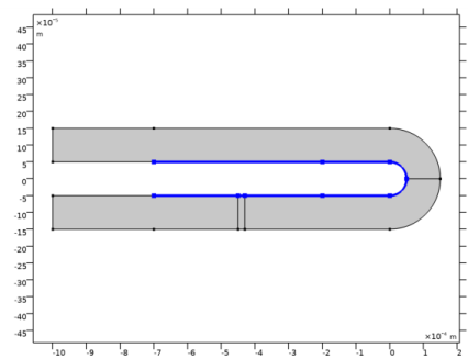
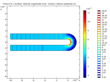
In the Settings window for 2D Plot Group, type Velocity and Electric Potential (Original Channel) in the Label text field.
Surface 1
1
Right-click Velocity and Electric Potential (Original Channel) and choose Surface.
2
In the Settings window for Surface, locate the Expression section.
3
In the Expression text field, type spf.U.
Contour 1
1
In the Model Builder window, right-click Velocity and Electric Potential (Original Channel) and choose Contour.
2
In the Settings window for Contour, locate the Levels section.
3
In the Total levels text field, type 30.
4
In the Velocity and Electric Potential (Original Channel) toolbar, click  Plot.
Concentration (Original Channel)
1
In the Home toolbar, click  Add Plot Group and choose 2D Plot Group.
2
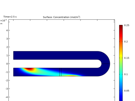
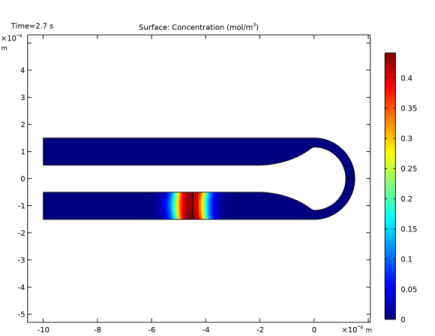
In the Settings window for 2D Plot Group, type Concentration (Original Channel) in the Label text field.
3
Locate the Data section. From the Time (s) list, choose 2.5.
Surface 1
1
Right-click Concentration (Original Channel) and choose Surface.
2
In the Settings window for Surface, click Replace Expression in the upper-right corner of the Expression section. From the menu, choose Component 1 (comp1)>Transport of Diluted Species>Species c>c - Concentration - mol/m³.
3
In the Concentration (Original Channel) toolbar, click  Plot.
Add Study
1
In the Home toolbar, click  Add Study to open the Add Study window.
2
Go to the Add Study window.
3
Find the Physics interfaces in study subsection. In the table, clear the Solve check box for Transport of Diluted Species (tds).
4
Find the Studies subsection. In the Select Study tree, select General Studies>Stationary.
5
Click Add Study in the window toolbar.
6
In the Home toolbar, click  Add Study to close the Add Study window.
Study 2
Step 1: Stationary
Minimize the difference in time needed for fluid to travel along the inner and outer edges of the channel.
1
In the Model Builder window, click Study 2.
2
In the Settings window for Study, type Shape Optimization Study in the Label text field.
3
Locate the Study Settings section. Clear the Generate default plots check box.
Optimization
1
In the Study toolbar, click  Optimization.
2
In the Settings window for Optimization, locate the Optimization Solver section.
3
From the Method list, choose BOBYQA.
4
Locate the Objective Function section. In the table, enter the following settings:
5
Locate the Control Variables and Parameters section. Click  Add.
6
7
8
9
10
11
12
13
14
15
In the Study toolbar, click  Compute.
Results
Velocity and Electric Potential (Optimized Channel)
1
In the Home toolbar, click  Add Plot Group and choose 2D Plot Group.
2
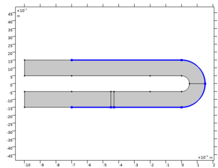
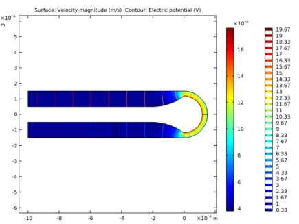
In the Settings window for 2D Plot Group, type Velocity and Electric Potential (Optimized Channel) in the Label text field.
3
Locate the Plot Settings section. From the Frame list, choose Spatial  (x, y, z).
4
Locate the Data section. From the Dataset list, choose Shape Optimization Study/Solution 3 (sol3).
Surface 1
1
Right-click Velocity and Electric Potential (Optimized Channel) and choose Surface.
2
In the Settings window for Surface, click Replace Expression in the upper-right corner of the Expression section. From the menu, choose Component 1 (comp1)>Creeping Flow>Velocity and pressure>spf.U - Velocity magnitude - m/s.
Contour 1
1
In the Model Builder window, right-click Velocity and Electric Potential (Optimized Channel) and choose Contour.
2
In the Settings window for Contour, locate the Levels section.
3
In the Total levels text field, type 30.
4
In the Velocity and Electric Potential (Optimized Channel) toolbar, click  Plot.
Add Study
1
In the Home toolbar, click  Add Study to open the Add Study window.
2
Go to the Add Study window.
3
Find the Physics interfaces in study subsection. In the table, clear the Solve check boxes for Electric Currents (ec) and Creeping Flow (spf).
4
Find the Studies subsection. In the Select Study tree, select General Studies>Time Dependent.
5
Click Add Study in the window toolbar.
6
In the Home toolbar, click  Add Study to close the Add Study window.
Optimized Channel Verification
1
In the Model Builder window, click Study 3.
2
In the Settings window for Study, type Optimized Channel Verification in the Label text field.
Step 1: Time Dependent
1
In the Model Builder window, under Optimized Channel Verification click Step 1: Time Dependent.
2
In the Settings window for Time Dependent, locate the Study Settings section.
3
In the Output times text field, type range(0,0.1,3.5).
4
From the Tolerance list, choose User controlled.
5
In the Relative tolerance text field, type 0.001.
6
Click to expand the Values of Dependent Variables section. Find the Initial values of variables solved for subsection. From the Settings list, choose User controlled.
7
From the Method list, choose Solution.
8
From the Study list, choose Shape Optimization Study, Stationary.
9
Find the Values of variables not solved for subsection. From the Settings list, choose User controlled.
10
From the Method list, choose Solution.
11
From the Study list, choose Shape Optimization Study, Stationary.
12
In the Model Builder window, click Optimized Channel Verification.
13
In the Settings window for Study, locate the Study Settings section.
14
Clear the Generate default plots check box.
15
In the Home toolbar, click  Compute.
Results
Concentration (Optimized Channel)
1
In the Home toolbar, click  Add Plot Group and choose 2D Plot Group.
2
In the Settings window for 2D Plot Group, type Concentration (Optimized Channel) in the Label text field.
3
Locate the Data section. From the Dataset list, choose Optimized Channel Verification/Solution 6 (sol6).
4
From the Time (s) list, choose 2.7.
Surface 1
1
Right-click Concentration (Optimized Channel) and choose Surface.
2
In the Settings window for Surface, click Replace Expression in the upper-right corner of the Expression section. From the menu, choose Component 1 (comp1)>Transport of Diluted Species>Species c>c - Concentration - mol/m³.
3
In the Concentration (Optimized Channel) toolbar, click  Plot.
Plot the average concentration in the detector for the original and optimized channels.
Average Concentration in Detector
1
In the Home toolbar, click  Add Plot Group and choose 1D Plot Group.
2
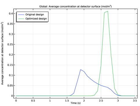
In the Settings window for 1D Plot Group, type Average Concentration in Detector in the Label text field.
Global 1
1
Right-click Average Concentration in Detector and choose Global.
2
In the Settings window for Global, locate the y-Axis Data section.
3
4
Click to expand the Legends section. From the Legends list, choose Manual.
5
Global 2
1
Right-click Global 1 and choose Duplicate.
2
In the Settings window for Global, locate the Data section.
3
From the Dataset list, choose Optimized Channel Verification/Solution 6 (sol6).
4
Click to expand the Title section. From the Title type list, choose None.
5
Locate the Legends section. In the table, enter the following settings:
Average Concentration in Detector
1
In the Model Builder window, click Average Concentration in Detector.
2
In the Settings window for 1D Plot Group, locate the Legend section.
3
From the Position list, choose Upper left.
Compare the original and optimized channels using animation.
Animation 1
1
In the Results toolbar, click  Animation and choose File.
2
In the Settings window for Animation, locate the Target section.
3
From the Target list, choose Player.
4
Locate the Scene section. From the Subject list, choose Concentration (Original Channel).
5
Right-click Animation 1 and choose Play.
Animation 2
1
In the Results toolbar, click  Animation and choose File.
2
In the Settings window for Animation, locate the Target section.
3
From the Target list, choose Player.
4
Locate the Scene section. From the Subject list, choose Concentration (Optimized Channel).
5
Right-click Animation 2 and choose Play.