Transformation Diagram Computation

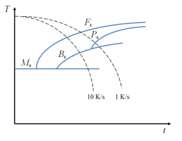
During quenching of steel, the austenite decomposes into destination phases such as ferrite, pearlite, bainite, and martensite. The resulting phase composition depends to a large extent on the temperature history, and also on the chemical composition and austenite grain size. A common way to illustrate the phase transformation characteristics is to use transformation diagrams. Two of the most commonly used diagram types are the CCT (continuous cooling transformation) and the TTT (time-temperature transformation) diagrams. In the former, the austenitized material is cooled at a constant temperature rate, while in the latter, the material is kept at a constant temperature. Figure 1 shows an example CCT diagram, with temperature on the vertical axis, and logarithmic time on the horizontal. Fs, Ps, and Bs represent the start temperatures, at a given cooling rate, for the formation of, respectively, ferrite, pearlite, and bainite. The example CCT diagram shows that a cooling rate of 10 K/s is sufficient to suppress the formation of pearlite, whereas 1 K/s is not.

Figure 1: A CCT diagram.

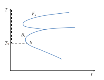
A TTT diagram differs from a CCT diagram in that the austenite is rapidly cooled to a given initial temperature T0, and then kept at that temperature, see Figure 2. This is performed for a range of start temperatures, and the transformation curves are constructed from the different times required to form a given phase. In a practical quenching situation, it is unlikely that material points will experience either of the two temperature histories that the CCT and TTT diagrams use, and instead experience varying temperature rates. Nevertheless, the diagrams can give useful insights into the phase transformation behavior of a certain material.

Figure 2: A TTT diagram.

In this model, CCT and TTT diagrams are constructed from a set of phase-transformation model data using the methods described above.

Model Definition

In order to compute transformation diagrams, no geometry is required, and suitable temperature histories can be accomplished without the need for a full heat-transfer analysis. The temperature is imposed as a parameter in the analysis. A number of parameters are used to compute the CCT and TTT diagrams. The diagrams are computed over a range of temperatures bounded by a lowest and a highest temperature. In the case of the CCT diagram computation, the cooling rate is additionally bounded by a lowest and a highest rate. The time-temperature combinations that illustrate the start of transformation in the CCT and TTT diagrams are obtained when a given phase reaches a defined (small) fraction. Table 1 shows these parameters.

Table 1: Parameters Used in the model definition.
Name	Value	Description
highT	900 °C	Highest transformation temperature
lowT	100 °C	Lowest transformation temperature
startFraction	0.01	Phase fraction indicating transformation start
highRate	100 K/s	Highest cooling rate for CCT
lowRate	0.01 K/s	Lowest cooling rate for CCT

Phase Transformations

For simplicity, the model only considers austenite decomposition into a combination of ferrite and bainite, but it can straightforwardly be extended to include other destination phases as well.

Austenite to Ferrite

The phase transformation is modeled using the Leblond-Devaux phase transformation model. The temperature dependent functions describing this transformation are given in Table 2.

Table 2: Austenite to Ferrite, Temperature dependent functions.
Temperature (°C)	K (1/s)	L (1/s)
550	0
600		0
620	0.002	0.0002
700	0.001
750	0
800		0.002
1000		0.002

Austenite to Bainite

The phase transformation is modeled using the Leblond–Devaux phase transformation model. Compared to the ferritic transformation, the bainitic transformation is active at lower temperatures. The temperature dependent functions describing the bainitic transformation are given in Table 3.

Table 3: Austenite to Bainite, Temperature dependent functions.
Temperature (°C)	K (1/s)	L (1/s)
380	0
400	0.0005	0
490	0.005
500		0.0002
580	0.00005	0.002
600	0	0.002

Note that the tabulated values are example values that define ferritic and bainitic transformations. Variations in alloying elements of the steel would cause the functions to be different.

Results and Discussion

The computed CCT is shown in Figure 3. Three cooling curves are shown, corresponding to the cooling rates 100 K/s, 10 K/s, and 1 K/s. The CCT diagram shows the time and temperature when a phase begins to form, given a cooling rate. In this example, a cooling rate of 10 K/s causes bainite to form after about 40 seconds, and at a temperature of 520 °C. At a rate of 100 K/s, neither ferrite nor bainite form. Note that in practice, this type of very rapid cooling would be used to obtain a martensitic structure, because the martensitic transformation only depends on the undercooling below the martensite start temperature, and not on time. The diffusionless martensitic transformation is not considered here.

If an experimentally obtained CCT diagram exists, it can be compared to the computed version to calibrate and verify the temperature dependent functions that describe each phase transformation. What complicates any calibration procedure is that the formation of one destination phase (such as ferrite) reduces the available fraction of source phase (austenite) to form other destination phases (such as bainite). The phase transformations are intrinsically coupled, and it is difficult to treat one phase transformation separate from another. An experimentally obtained CCT diagram is therefore best compared to a computed CCT diagram that includes all relevant phase transformations.

Figure 3: Computed CCT diagram showing the curves for 1% formed fraction of ferrite and bainite.

The computed TTT diagram is shown in Figure 4. Unlike the CCT diagram, the TTT diagram is more straightforwardly used to calibrate phase transformation models. In contrast, the CCT diagram is more likely to realistically represent a quenching process. During a process of constant temperature, a certain phase transformation can be calibrated more easily, as the temperature dependent functions in Table 2 and Table 3 become constants. The CCT and TTT diagrams are computed using the same set of data for the phase transformations involved.