PDF

Piezoelectric Rate Gyroscope
Introduction
This model shows how to analyze a tuning fork based piezoelectric rate gyroscope. The reverse piezoelectric effect is used to drive an in-plane tuning fork mode. This mode is coupled to an out of plane mode by the Coriolis force and the resulting out of plane motion is sensed by the direct piezoelectric effect. The geometry of the tuning forks is designed so that the eigenfrequencies of the nearby modes are separated in frequency space. The frequency response of the system is computed and the rotation rate sensitivity is evaluated. Note that the model focuses on the performance of the sensor in a uniformly rotating reference frame. The model is based on the detailed analysis of a similar device presented in Ref. 1.
Model Definition
Figure 1 shows the geometry of the device indicating the key features.
Figure 1: Device geometry showing the plane of symmetry through the center of the device and the key components of the gyroscope.
The packaging and fabrication of the device is discussed in Ref. 1. Here we provide a simple explanation of its principle of operation when operated in a rotating frame with no angular acceleration (Ref. 1 discusses the effects of an angular acceleration on the frequency response of the device in more detail). The gyroscope can be thought of as two tuning forks, coupled together by a suspension structure. The suspension is anchored to the package of the device which is in turn attached to the rotating object. The drive tines are driven close to their resonance in an in-plane mode, as shown in Figure 2. The sense tines are designed to have a resonance at a nearby, but distinct, frequency with a significant out of plane component to their motion, as shown in Figure 3. As the drive mode vibrates in the in-plane direction within the rotating frame a Coriolis body force acts on the structure which excites the out of plane sense mode. The Coriolis force (Fcor) is given by:
Where ρ is the density of the material, Ω is the angular acceleration of the frame and u is the local velocity of the structure. From the above equation it is clear that the Coriolis force is maximal when the angular velocity of the frame is parallel to the long in-plane axis of the gyroscope structure. In this case the resulting force is in the out of plane direction and produces a corresponding out of plane motion of the drive tines. This motion causes reaction moments in the supporting suspension which in turn transfers these moments to the sense tines — driving the sense mode. Note that in this model the angular velocity vector is assumed to be parallel to the long axis of the device.
The tines are fabricated from single crystal quartz wafers with the crystallographic Z-axis aligned parallel to the normal of the wafer plane. The details of the design are discussed in Ref. 1, but the critical point is that the electrodes are patterned in such a way that both in-plane and in-phase out-of-plane motion of the sense tines is not detected by the sense electrodes. This leads to the rejection of unwanted signals in the output of the sensor.
In general, for resonant structures like this model, a very fine mesh is required to achieve accurate frequency response results. In the interest of saving time, we choose to use a relatively coarse mesh for this tutorial. As a result the resonant peak will shift if a more refined mesh is used instead.
Results and Discussion
Figure 2 shows the eigenmode corresponding to the drive mode and Figure 3 shows that corresponding to the sense mode. Both the in-plane and out-of-plane motions of these modes are shown separately in the figures.
Figure 2: Drive mode, showing both in-plane motion (right) and out-of-plane motion (left). Note that the amplitude scale is arbitrary — only the relative value of the in-plane and out-of-plane displacements has physical significance.
Figure 3: Sense mode, showing out-of-plane motion (left) and in-plane motion (right). Note that the amplitude scale is arbitrary — only the relative value of the in-plane and out-of-plane displacements has physical significance.
Figure 4: Sense voltage vs. drive frequency with an applied sinusoidal drive voltage of amplitude 2 V and an angular acceleration of 64 deg/s.
Figure 5: Sense voltage vs. angular acceleration at a drive voltage amplitude of 2 V and a frequency of 8396 Hz.
Figure 4 shows the response of the device as the frequency of the drive voltage waveform is varied. A clear peak in the response close to the drive frequency, at approximately 8396 Hz is apparent. This is the optimum drive frequency for the device. Figure 5 shows the sense voltage against the angular acceleration with a 2 V drive voltage at a frequency close to this optimum. As expected the response of the sensor is linear, with a sensitivity of approximately 0.015 mV /(deg/s).
Reference
1. S.D. Senturia, “A Piezoelectric Rate Gyroscope,” Microsystem Design, chapter 21, Springer, 2000.
Application Library path: MEMS_Module/Piezoelectric_Devices/piezoelectric_rate_gyroscope
Modeling Instructions
From the File menu, choose New.
New
In the New window, click  Model Wizard.
Model Wizard
1
In the Model Wizard window, click  3D.
2
In the Select Physics tree, select Structural Mechanics>Electromagnetics-Structure Interaction>Piezoelectricity>Piezoelectricity, Solid.
3
Click Add.
4
Click  Study.
5
In the Select Study tree, select Preset Studies for Selected Multiphysics>Eigenfrequency.
6
Geometry 1
Add some global parameters.
Global Definitions
Parameters 1
1
In the Model Builder window, under Global Definitions click Parameters 1.
2
In the Settings window for Parameters, locate the Parameters section.
3
Build a symmetric mesh for this model so that the numerical result for no rotation will be very close to the expected null result. To prevent the symmetry of the mesh from being broken, clear the Avoid inverted elements by curving interior domain elements check box.
Component 1 (comp1)
1
In the Model Builder window, click Component 1 (comp1).
2
In the Settings window for Component, locate the General section.
3
Find the Mesh frame coordinates subsection. Clear the Avoid inverted elements by curving interior domain elements check box.
Import the geometry from file.
Geometry 1
1
In the Model Builder window, under Component 1 (comp1) click Geometry 1.
2
In the Settings window for Geometry, locate the Units section.
3
From the Length unit list, choose mm.
4
In the Geometry toolbar, click  Insert Sequence.
5
6
In the Geometry toolbar, click  Build All.
7
Click the  Zoom Extents button in the Graphics toolbar.
The Adaptive Frequency Sweep study step will generate a high resolution frequency sweep. To avoid large file size, create an "explicit selection" to store solution data only on the external surfaces of the modeling domain.
Definitions
External surfaces
1
In the Definitions toolbar, click  Explicit.
2
In the Settings window for Explicit, locate the Input Entities section.
3
Select the All domains check box.
4
Locate the Output Entities section. From the Output entities list, choose Adjacent boundaries.
5
In the Label text field, type External surfaces.
Add the built-in quartz material.
Add Material
1
In the Home toolbar, click  Add Material to open the Add Material window.
2
Go to the Add Material window.
3
In the tree, select Piezoelectric>Quartz LH (1978 IEEE).
4
Click Add to Component in the window toolbar.
5
In the Home toolbar, click  Add Material to close the Add Material window.
Set up the physics.
Solid Mechanics (solid)
Piezoelectric Material 1
In the Model Builder window, under Component 1 (comp1)>Solid Mechanics (solid) click Piezoelectric Material 1.
Mechanical Damping 1
1
In the Physics toolbar, click  Attributes and choose Mechanical Damping.
2
In the Settings window for Mechanical Damping, locate the Damping Settings section.
3
From the Damping type list, choose Isotropic loss factor.
4
From the ηs list, choose User defined. In the associated text field, type 5e-5.
Anchor the circular region underneath the structure.
Fixed Constraint 1
1
In the Physics toolbar, click  Boundaries and choose Fixed Constraint.
2
Add rotating frame physics.
Rotating Frame 1
1
In the Physics toolbar, click  Domains and choose Rotating Frame.
2
In the Settings window for Rotating Frame, locate the Domain Selection section.
3
From the Selection list, choose All domains.
4
Locate the Rotating Frame section. From the Axis of rotation list, choose y-axis.
5
In the Ω text field, type va.
6
Locate the Frame Acceleration Effect section. Select the Coriolis force check box.
Electrostatics (es)
Add boundary conditions for the drive and sense electrodes.
1
In the Model Builder window, under Component 1 (comp1) click Electrostatics (es).
Drive Terminal 1
1
In the Physics toolbar, click  Boundaries and choose Terminal.
2
In the Settings window for Terminal, type Drive Terminal 1 in the Label text field.
3
4
Locate the Terminal section. From the Terminal type list, choose Voltage.
Drive Terminal 2
1
In the Physics toolbar, click  Boundaries and choose Terminal.
2
In the Settings window for Terminal, type Drive Terminal 2 in the Label text field.
3
4
Locate the Terminal section. From the Terminal type list, choose Voltage.
5
In the V0 text field, type -1.
Sense Terminal 1
1
In the Physics toolbar, click  Boundaries and choose Terminal.
2
In the Settings window for Terminal, type Sense Terminal 1 in the Label text field.
3
Sense Terminal 2
1
In the Physics toolbar, click  Boundaries and choose Terminal.
2
In the Settings window for Terminal, type Sense Terminal 2 in the Label text field.
3
Build a symmetric mesh for this model so that the numerical result for no rotation will be very close to the expected null result. To save computation time and to reduce file size, a relatively coarse mesh is used.
Mesh 1
1
In the Model Builder window, under Component 1 (comp1) click Mesh 1.
2
In the Settings window for Mesh, locate the Mesh Settings section.
3
From the Sequence type list, choose User-controlled mesh.
Size
1
In the Model Builder window, under Component 1 (comp1)>Mesh 1 click Size.
2
In the Settings window for Size, locate the Element Size section.
3
From the Predefined list, choose Finer.
4
Click the Custom button.
5
Locate the Element Size Parameters section. In the Maximum element size text field, type tQz/4.
6
In the Minimum element size text field, type tQz/12.
Free Tetrahedral 1
1
In the Model Builder window, click Free Tetrahedral 1.
2
In the Settings window for Free Tetrahedral, locate the Domain Selection section.
3
From the Geometric entity level list, choose Domain.
4
Copy Domain 1
1
In the Model Builder window, right-click Mesh 1 and choose More Operations>Copy Domain.
2
3
In the Settings window for Copy Domain, locate the Destination Domains section.
4
Select the  Activate Selection toggle button.
5
6
In the Home toolbar, click  Build Mesh.
Set up the eigenfrequency study to solve for the eigenmodes.
Eigenmodes
1
In the Model Builder window, click Study 1.
2
In the Settings window for Study, type Eigenmodes in the Label text field.
Step 1: Eigenfrequency
1
In the Model Builder window, under Eigenmodes click Step 1: Eigenfrequency.
2
In the Settings window for Eigenfrequency, locate the Study Settings section.
3
Select the Desired number of eigenfrequencies check box.
4
5
In the Search for eigenfrequencies around text field, type 3e3.
6
From the Eigenfrequency search method around shift list, choose Larger real part.
7
In the Home toolbar, click  Compute.
Results
Mode Shape (solid)
The default mode shape plot shows a surface plot of the displacement magnitude. To provide a deeper insight into the mode shapes, plot the x and z displacements in two separate surface plots instead.
Change the default surface plot to plot the x displacement.
Surface 1
1
In the Model Builder window, expand the Mode Shape (solid) node, then click Surface 1.
2
In the Settings window for Surface, locate the Expression section.
3
In the Expression text field, type u.
Duplicate the surface plot to plot the z displacement.
Surface 2
1
Right-click Results>Mode Shape (solid)>Surface 1 and choose Duplicate.
2
In the Settings window for Surface, locate the Expression section.
3
In the Expression text field, type w.
4
Locate the Coloring and Style section. From the Color table list, choose RainbowLight.
Deformation
1
In the Model Builder window, expand the Surface 2 node, then click Deformation.
2
In the Settings window for Deformation, locate the Expression section.
3
In the x component text field, type -w_f*1.3.
4
In the y component text field, type 0.
5
In the z component text field, type 0.
6
Locate the Scale section. Select the Scale factor check box.
7
Mode Shape (solid)
Turn on color legend to see the relative amplitude of the x and z displacements.
1
In the Model Builder window, click Mode Shape (solid).
2
In the Settings window for 3D Plot Group, locate the Color Legend section.
3
Select the Show legends check box.
4
From the Position list, choose Alternating.
Plot the mode shape of the drive mode.
5
Locate the Data section. From the Eigenfrequency (Hz) list, choose 8396.2+0.20848i.
6
In the Mode Shape (solid) toolbar, click  Plot.
7
Click the  Zoom Extents button in the Graphics toolbar.
Plot the sense mode, which is at a higher frequency.
8
From the Eigenfrequency (Hz) list, choose 10630+0.26346i.
9
In the Mode Shape (solid) toolbar, click  Plot.
10
Click the  Zoom Extents button in the Graphics toolbar.
Set up and solve an Adaptive Frequency Sweep study, which is optimized for resolving narrow resonant peaks without excessive computation.
Add Study
1
In the Home toolbar, click  Add Study to open the Add Study window.
2
Go to the Add Study window.
3
Find the Studies subsection. In the Select Study tree, select Empty Study.
4
Click Add Study in the window toolbar.
5
In the Home toolbar, click  Add Study to close the Add Study window.
Frequency Response
1
In the Settings window for Study, type Frequency Response in the Label text field.
2
Locate the Study Settings section. Clear the Generate default plots check box.
Adaptive Frequency Sweep
1
In the Study toolbar, click  Study Steps and choose Frequency Domain>Adaptive Frequency Sweep.
2
In the Settings window for Adaptive Frequency Sweep, locate the Study Settings section.
3
In the Frequencies text field, type range(-1.3,0.02,1.3)+8396.2.
4
From the AWE expression type list, choose User controlled.
5
To reduce file size, only store solution data on the external surfaces.
6
Locate the Values of Dependent Variables section. Find the Store fields in output subsection. From the Settings list, choose For selections.
7
Under Selections, click  Add.
8
In the Add dialog box, select External surfaces in the Selections list.
9
10
In the Study toolbar, click  Compute.
Create plots to visualize the frequency response of the displacement and the sense voltage.
Results
Frequency Response: Displacement
1
Right-click Mode Shape (solid) and choose Duplicate.
2
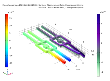
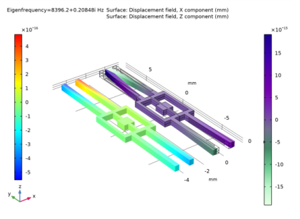
In the Settings window for 3D Plot Group, type Frequency Response: Displacement in the Label text field.
3
Locate the Data section. From the Dataset list, choose Frequency Response/Solution 2 (sol2).
4
In the Frequency Response: Displacement toolbar, click  Plot.
Frequency Response: Sense Voltage
1
In the Home toolbar, click  Add Plot Group and choose 1D Plot Group.
2
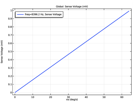
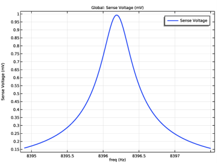
In the Settings window for 1D Plot Group, type Frequency Response: Sense Voltage in the Label text field.
3
Locate the Data section. From the Dataset list, choose Frequency Response/Solution 2 (sol2).
Sense Voltage
1
Right-click Frequency Response: Sense Voltage and choose Global.
2
In the Settings window for Global, type Sense Voltage in the Label text field.
3
Locate the y-Axis Data section. In the table, enter the following settings:
4
Click to expand the Coloring and Style section. In the Width text field, type 2.
5
In the Frequency Response: Sense Voltage toolbar, click  Plot.
Add a study and make a plot to evaluate the sensitivity of the device.
Add Study
1
In the Home toolbar, click  Add Study to open the Add Study window.
2
Go to the Add Study window.
3
Find the Studies subsection. In the Select Study tree, select General Studies>Frequency Domain.
4
Click Add Study in the window toolbar.
5
In the Home toolbar, click  Add Study to close the Add Study window.
Study 3
Step 1: Frequency Domain
1
In the Settings window for Frequency Domain, locate the Study Settings section.
2
In the Frequencies text field, type 8396.2.
3
Click to expand the Study Extensions section. Select the Auxiliary sweep check box.
4
5
6
In the Model Builder window, click Study 3.
7
In the Settings window for Study, locate the Study Settings section.
8
Clear the Generate default plots check box.
9
In the Label text field, type Sensitivity.
10
In the Home toolbar, click  Compute.
Results
Sensitivity: Sense Voltage vs. Angular Velocity
1
In the Model Builder window, right-click Frequency Response: Sense Voltage and choose Duplicate.
2
In the Settings window for 1D Plot Group, locate the Data section.
3
From the Dataset list, choose Sensitivity/Solution 3 (sol3).
4
Locate the Legend section. From the Position list, choose Upper left.
5
In the Label text field, type Sensitivity: Sense Voltage vs. Angular Velocity.
Sense Voltage
1
In the Model Builder window, expand the Sensitivity: Sense Voltage vs. Angular Velocity node, then click Sense Voltage.
2
In the Settings window for Global, locate the x-Axis Data section.
3
From the Unit list, choose deg/s.
4
In the Sensitivity: Sense Voltage vs. Angular Velocity toolbar, click  Plot.