PDF

A Piezoelectric Micropump
Introduction
This tutorial model is kindly provided by Riccardo Vietri, James Ransley, and Andrew Spann at Veryst Engineering, LLC. Piezoelectric micropumps are frequently used in medical applications because of their ability to precisely control the metering of very small volumes of fluids or gases. This example shows how to simulate a simple, non-resonant micropump, suitable for low flow rate applications. The model demonstrates the combination of piezoelectric materials with a fluid-structure interaction, and also illustrates the use of a simple velocity-dependent formula to account for the presence of valves on the inlet and outlet boundaries.
Model Definition
The model geometry consists of an annular piezoelectric actuator on top of the fluid domain which is connected to a flexible membrane (highlighted in Figure 1). Due to the symmetry of the physics, only half of the geometry needs to be included. The fluid flows out when a voltage is applied, and the actuator expands. The circumference of the membrane is fixed as the actuator moves, and it imposes a force on the fluid beneath it, pulling in fluid from the left and pushing fluid out of the channel on the right.
Figure 1: The geometry of the piezoelectric micropump. The membrane is highlighted.
In a real micropump, a stacked piezoelectric actuator would be employed with many separate piezoelectric layers and electrical contacts. For the purposes of this model, neglect the stiffness of the thin metal layers and model the actuator as a monolithic block of piezoelectric. Consequently, apply a high potential difference of 1500 V across the entire piezoelectric. This corresponds to an electric field of 0.2 V/µm. The voltage required in a real device would depend on the thickness of each layer in the stacked actuator.
The inlet and outlet work by employing check valves to ensure a one-way flow. In the model the valve is represented by a simple boundary condition based on K-factor piping losses, where the losses are high when flowing against the valve and low when flowing in the direction of operation. The back pressure resulting from the valve is represented by the following equation:
(1)
where uav is the average velocity of the fluid normal to the boundary, ρ is the fluid density and A is a dimensionless constant that changes magnitude depending on the sign of uav. The back pressure is applied as a normal stress at the end of a short length of pipe - which ensures that the fluid flow in the domain is realistic, despite this approximate boundary condition. This boundary condition can be employed to represent a simple fluid valve or diode. The constants used for the outlet boundary are reversed with respect to those used in the inlet, representing a different orientation of a similar valve. This encourages flow through the pump in the desired direction. To represent a low resistance valve (such as a simple flapper valve), set A to 5,000 for closed condition and to 0.1 for the open condition. Careful tuning of these values and potentially refinement of this model would be desirable in a real application.
To save computation time for the purposes of this example, a relatively coarse mesh is used, as shown in the figure below.
Figure 2: The mesh used in the model. Note the fluid boundary layers next to the highlighted fluid walls.
Results and Discussion
Figure 3 shows the inlet and outlet flow rates and confirms the conservation of fluid volume within the device. The drive voltage is ramped up during the first 3/4 of the actuation period. Afterwards, a consistent time periodic flow is quickly established. The difference in inlet and outlet flow matches the volume of the fluid displaced by the membrane due to the piezoelectric stroke, confirming the volume conservation.
Figure 3: Flow rates and volume conservation.
The time integrated flows into the inlet and out of the outlet are calculated using a global ODE and are shown in Figure 4. The net flow through the pump in 0.05 s is 1.8 µL, corresponding to 36 µL/s or 2.16 ml/min. This is typical for such a nonresonant design.
Figure 4: Net fluid flow through the inlet and the outlet over time, computed using a global ordinary differential equation.
Figure 5 shows the flow through the inlet (left) and outlet (right) when fluid is being drawn into the chamber, whilst Figure 6 shows the case when fluid is being forced out of the chamber.
Figure 5: Velocity (base 10 logarithm in mm/s) when fluid is being drawn through the inlet.
Figure 6: Velocity (base 10 logarithm in mm/s) when fluid is being pushed through the outlet.
Figure 7 and Figure 8 show the fluid streamlines in the corresponding cases.
Figure 7: Flow streamlines when fluid is being drawn through the inlet. The color shows the base 10 logarithm of the velocity in mm/s.
Figure 8: Flow streamlines when fluid is being pushed through the outlet. The color shows the base 10 logarithm of the velocity in mm/s.
Application Library path: MEMS_Module/Fluid-Structure_Interaction/piezoelectric_micropump
Modeling Instructions
From the File menu, choose New.
New
In the New window, click  Model Wizard.
Model Wizard
1
In the Model Wizard window, click  3D.
In addition to piezoelectricity and laminar flow, a global equation will be used to keep track of the total flow through the inlet and the outlet.
2
In the Select Physics tree, select Structural Mechanics>Electromagnetics-Structure Interaction>Piezoelectricity>Piezoelectricity, Solid.
3
Click Add.
4
In the Select Physics tree, select Fluid Flow>Single-Phase Flow>Laminar Flow (spf).
5
Click Add.
6
In the Select Physics tree, select Mathematics>ODE and DAE Interfaces>Global ODEs and DAEs (ge).
7
Click Add.
8
Click  Study.
9
In the Select Study tree, select General Studies>Time Dependent.
10
Geometry 1
The Model Wizard starts the COMSOL Desktop at the Geometry node. Take the opportunity to set the length unit to mm for convenience.
1
In the Model Builder window, under Component 1 (comp1) click Geometry 1.
2
In the Settings window for Geometry, locate the Units section.
3
From the Length unit list, choose mm.
Enter some global parameters. The expression containing the parameter r_inlet appears red initially and turns to black once r_inlet is defined.
Global Definitions
Parameters 1
1
In the Model Builder window, under Global Definitions click Parameters 1.
2
In the Settings window for Parameters, locate the Parameters section.
3
Build the geometry. We will model only half of the device using the symmetry of the problem. Use Form Assembly with Create imprints to allow different meshes in the solid and the fluid domains, while still creating a matching pair of surfaces for the solid-fluid interface.
The fluid chamber is a simple block.
Geometry 1
Block 1 - Fluid Chamber
1
In the Geometry toolbar, click  Block.
2
In the Settings window for Block, type Block 1 - Fluid Chamber in the Label text field.
3
Locate the Size and Shape section. In the Width text field, type w_block.
4
In the Depth text field, type depth_block.
5
In the Height text field, type h_block-h_memb.
6
Locate the Position section. From the Base list, choose Center.
7
In the z text field, type -h_memb/2.
The piezoelectric stack is a hollow cylinder, which can be constructed by taking the difference between two cylinders.
Cylinder 1 - Piezo OD
1
In the Geometry toolbar, click  Cylinder.
2
In the Settings window for Cylinder, type Cylinder 1 - Piezo OD in the Label text field.
3
Locate the Size and Shape section. In the Radius text field, type OD/2.
4
In the Height text field, type t0*n.
5
Locate the Position section. In the z text field, type h_block/2.
Cylinder 2 - Piezo ID
1
Right-click Cylinder 1 - Piezo OD and choose Duplicate.
2
In the Settings window for Cylinder, type Cylinder 2 - Piezo ID in the Label text field.
3
Locate the Size and Shape section. In the Radius text field, type ID/2.
Difference 1 - Piezo
1
In the Geometry toolbar, click  Booleans and Partitions and choose Difference.
2
In the Settings window for Difference, type Difference 1 - Piezo in the Label text field.
3
4
Locate the Difference section. Find the Objects to subtract subsection. Select the  Activate Selection toggle button.
5
The actuated membrane is a simple cylinder, so are the inlet and outlet pipes.
Cylinder 3 - Membrane
1
In the Geometry toolbar, click  Cylinder.
2
In the Settings window for Cylinder, type Cylinder 3 - Membrane in the Label text field.
3
Locate the Size and Shape section. In the Radius text field, type r_memb.
4
In the Height text field, type h_memb.
5
Locate the Position section. In the z text field, type h_block/2-h_memb.
Cylinder 4 - Inlet
1
In the Geometry toolbar, click  Cylinder.
2
In the Settings window for Cylinder, type Cylinder 4 - Inlet in the Label text field.
3
Locate the Size and Shape section. In the Radius text field, type r_inlet.
4
In the Height text field, type h_exit.
5
Locate the Position section. In the x text field, type -(OD+ID)/4.
6
In the z text field, type -h_block/2-h_exit.
Cylinder 5 - Outlet
1
Right-click Cylinder 4 - Inlet and choose Duplicate.
2
In the Settings window for Cylinder, type Cylinder 5 - Outlet in the Label text field.
3
Locate the Size and Shape section. In the Radius text field, type r_outlet.
4
Locate the Position section. In the x text field, type (OD+ID)/4.
Use a workplane to divide the geometry to two symmetric parts and remove one of them.
Work Plane 1 - Symmetry Plane
1
In the Geometry toolbar, click  Work Plane.
2
In the Settings window for Work Plane, type Work Plane 1 - Symmetry Plane in the Label text field.
3
Locate the Plane Definition section. From the Plane list, choose xz-plane.
Partition Objects 1 (par1)
1
In the Geometry toolbar, click  Booleans and Partitions and choose Partition Objects.
2
3
Click in the Graphics window and then press Ctrl+A to select all objects.
4
In the Settings window for Partition Objects, locate the Partition Objects section.
5
From the Partition with list, choose Work plane.
Delete Entities 1 (del1)
1
In the Model Builder window, right-click Geometry 1 and choose Delete Entities.
2
In the Settings window for Delete Entities, locate the Entities or Objects to Delete section.
3
From the Geometric entity level list, choose Domain.
4
On the object par1(1), select Domain 1 only.
5
On the object par1(2), select Domain 1 only.
6
On the object par1(3), select Domain 1 only.
7
On the object par1(4), select Domain 1 only.
8
On the object par1(5), select Domain 1 only.
Unite the solid and fluid parts of the geometry separately with a selection defined for each, and then finalize the geometry using Form Assembly.
Union 1 - Solid
1
In the Geometry toolbar, click  Booleans and Partitions and choose Union.
2
In the Settings window for Union, type Union 1 - Solid in the Label text field.
3
Select the objects del1(2) and del1(5) only.
4
Locate the Selections of Resulting Entities section. Select the Resulting objects selection check box.
Union 2 - Fluid
1
In the Geometry toolbar, click  Booleans and Partitions and choose Union.
2
In the Settings window for Union, type Union 2 - Fluid in the Label text field.
3
Select the objects del1(1), del1(3), and del1(4) only.
4
Locate the Selections of Resulting Entities section. Select the Resulting objects selection check box.
Form Union (fin)
1
In the Model Builder window, under Component 1 (comp1)>Geometry 1 click Form Union (fin).
2
In the Settings window for Form Union/Assembly, locate the Form Union/Assembly section.
3
From the Action list, choose Form an assembly.
4
Select the Create imprints check box.
5
In the Geometry toolbar, click  Build All.
Create selections for the subsequent settings. First define the piezoelectric stack domain using a box selection.
Definitions
Box 1 - Piezo
1
In the Definitions toolbar, click  Box.
2
In the Settings window for Box, type Box 1 - Piezo in the Label text field.
3
Locate the Box Limits section. In the x minimum text field, type h_block/2-h_memb/2.
4
Locate the Output Entities section. From the Include entity if list, choose Entity inside box.
5
Locate the Box Limits section. In the x minimum text field, type -inf.
6
In the z minimum text field, type h_block/2-h_memb/2.
The membrane domain is given by the difference between the solid domain and the piezoelectric stack.
Difference 1 - Membrane
1
In the Definitions toolbar, click  Difference.
2
In the Settings window for Difference, type Difference 1 - Membrane in the Label text field.
3
Locate the Input Entities section. Under Selections to add, click  Add.
4
In the Add dialog box, select Union 1 - Solid in the Selections to add list.
5
6
In the Settings window for Difference, locate the Input Entities section.
7
Under Selections to subtract, click  Add.
8
In the Add dialog box, select Box 1 - Piezo in the Selections to subtract list.
9
Define the inlet and outlet boundaries using box selections.
Box 2 - Inlet
1
In the Definitions toolbar, click  Box.
2
In the Settings window for Box, type Box 2 - Inlet in the Label text field.
3
Locate the Geometric Entity Level section. From the Level list, choose Boundary.
4
Locate the Box Limits section. In the x maximum text field, type 0.
5
In the z maximum text field, type -h_block/2-h_exit/2.
6
Locate the Output Entities section. From the Include entity if list, choose Entity inside box.
Use wireframe rendering to see the inlet boundary selection better.
7
Click the  Wireframe Rendering button in the Graphics toolbar.
Box 3 - Outlet
1
Right-click Box 2 - Inlet and choose Duplicate.
2
In the Settings window for Box, type Box 3 - Outlet in the Label text field.
3
Locate the Box Limits section. In the x minimum text field, type 0.
4
In the x maximum text field, type Inf.
Use a box selection to define the symmetry plane.
Box 4 - Symmetry Plane
1
In the Definitions toolbar, click  Box.
2
In the Settings window for Box, type Box 4 - Symmetry Plane in the Label text field.
3
Locate the Geometric Entity Level section. From the Level list, choose Boundary.
4
Locate the Box Limits section. In the y maximum text field, type min(min(r_inlet,r_outlet),ID)/2.
5
Locate the Output Entities section. From the Include entity if list, choose Entity inside box.
Create a selection for the fluid walls by removing the symmetry plane and the in/outlets from the boundaries adjacent to the fluid. This selection can be used to create boundary layer mesh for the flow problem.
Adjacent 1 - All Fluid Boundaries
1
In the Definitions toolbar, click  Adjacent.
2
In the Settings window for Adjacent, type Adjacent 1 - All Fluid Boundaries in the Label text field.
3
Locate the Input Entities section. Under Input selections, click  Add.
4
In the Add dialog box, select Union 2 - Fluid in the Input selections list.
5
Difference 2 - Fluid Walls
1
In the Definitions toolbar, click  Difference.
2
In the Settings window for Difference, type Difference 2 - Fluid Walls in the Label text field.
3
Locate the Geometric Entity Level section. From the Level list, choose Boundary.
4
Locate the Input Entities section. Under Selections to add, click  Add.
5
In the Add dialog box, select Adjacent 1 - All Fluid Boundaries in the Selections to add list.
6
7
In the Settings window for Difference, locate the Input Entities section.
8
Under Selections to subtract, click  Add.
9
In the Add dialog box, select Box 2 - Inlet in the Selections to subtract list.
10
11
In the Settings window for Difference, locate the Input Entities section.
12
Under Selections to subtract, click  Add.
13
In the Add dialog box, select Box 3 - Outlet in the Selections to subtract list.
14
15
In the Settings window for Difference, locate the Input Entities section.
16
Under Selections to subtract, click  Add.
17
In the Add dialog box, select Box 4 - Symmetry Plane in the Selections to subtract list.
18
Create a selection for the membrane boundary to be used to keep track of the volume change of the fluid chamber.
Box 5
1
In the Definitions toolbar, click  Box.
2
In the Settings window for Box, locate the Geometric Entity Level section.
3
From the Level list, choose Boundary.
4
Locate the Box Limits section. In the x minimum text field, type -eps.
5
In the x maximum text field, type eps.
6
In the y minimum text field, type -eps.
7
In the y maximum text field, type eps.
8
In the z minimum text field, type h_block/2-h_memb-eps.
Intersection 1 - Fluid Membrane
1
In the Definitions toolbar, click  Intersection.
2
In the Settings window for Intersection, type Intersection 1 - Fluid Membrane in the Label text field.
3
Locate the Geometric Entity Level section. From the Level list, choose Boundary.
4
Locate the Input Entities section. Under Selections to intersect, click  Add.
5
In the Add dialog box, in the Selections to intersect list, choose Difference 2 - Fluid Walls and Box 5.
6
Finally select the top surface of the piezoelectric stack and the circumference of the membrane for the fixed constraint in the solid problem.
Explicit 1 - Fixed Boundaries
1
In the Definitions toolbar, click  Explicit.
2
In the Settings window for Explicit, type Explicit 1 - Fixed Boundaries in the Label text field.
3
Locate the Input Entities section. From the Geometric entity level list, choose Boundary.
4
Add material data to the corresponding selections.
Add Material
1
In the Home toolbar, click  Add Material to open the Add Material window.
2
Go to the Add Material window.
3
In the tree, select Built-in>Water, liquid.
4
Click Add to Component in the window toolbar.
5
In the tree, select Piezoelectric>Lead Zirconate Titanate (PZT-5H).
6
Click Add to Component in the window toolbar.
7
In the Home toolbar, click  Add Material to close the Add Material window.
Materials
Water, liquid (mat1)
1
In the Model Builder window, under Component 1 (comp1)>Materials click Water, liquid (mat1).
2
In the Settings window for Material, locate the Geometric Entity Selection section.
3
From the Selection list, choose Union 2 - Fluid.
Lead Zirconate Titanate (PZT-5H) (mat2)
1
In the Model Builder window, click Lead Zirconate Titanate (PZT-5H) (mat2).
2
In the Settings window for Material, locate the Geometric Entity Selection section.
3
From the Selection list, choose Box 1 - Piezo.
Membrane
1
In the Model Builder window, right-click Materials and choose Blank Material.
2
In the Settings window for Material, type Membrane in the Label text field.
3
Locate the Geometric Entity Selection section. From the Selection list, choose Difference 1 - Membrane.
At this point the set of properties shown for the user-defined membrane material is not as intended, because the physics selections haven’t been configured yet.
Set up the physics selections relevant for the material data.
Solid Mechanics (solid)
1
In the Model Builder window, under Component 1 (comp1) click Solid Mechanics (solid).
2
In the Settings window for Solid Mechanics, locate the Domain Selection section.
3
From the Selection list, choose Union 1 - Solid.
Piezoelectric Material 1
1
In the Model Builder window, under Component 1 (comp1)>Solid Mechanics (solid) click Piezoelectric Material 1.
2
In the Settings window for Piezoelectric Material, locate the Domain Selection section.
3
From the Selection list, choose Box 1 - Piezo.
Electrostatics (es)
1
In the Model Builder window, under Component 1 (comp1) click Electrostatics (es).
2
In the Settings window for Electrostatics, locate the Domain Selection section.
3
From the Selection list, choose Box 1 - Piezo.
Laminar Flow (spf)
1
In the Model Builder window, under Component 1 (comp1) click Laminar Flow (spf).
2
In the Settings window for Laminar Flow, locate the Domain Selection section.
3
From the Selection list, choose Union 2 - Fluid.
Now we are ready to enter the material properties for the membrane.
Materials
Membrane (mat3)
1
In the Model Builder window, under Component 1 (comp1)>Materials click Membrane (mat3).
2
In the Settings window for Material, locate the Material Contents section.
3
Continue setting up the physics. Add fixed constraint and symmetry boundary condition to solid mechanics, using the boundary selections defined earlier.
Solid Mechanics (solid)
In the Model Builder window, under Component 1 (comp1) click Solid Mechanics (solid).
Fixed Constraint 1
1
In the Physics toolbar, click  Boundaries and choose Fixed Constraint.
2
In the Settings window for Fixed Constraint, locate the Boundary Selection section.
3
From the Selection list, choose Explicit 1 - Fixed Boundaries.
Symmetry 1
1
In the Physics toolbar, click  Boundaries and choose Symmetry.
2
In the Settings window for Symmetry, locate the Boundary Selection section.
3
From the Selection list, choose Box 4 - Symmetry Plane.
Add electrical terminals to the top and bottom surfaces of the piezoelectric stack, using a terminal boundary condition on the top and a ground boundary condition at the bottom.
Electrostatics (es)
In the Model Builder window, under Component 1 (comp1) click Electrostatics (es).
Terminal 1
1
In the Physics toolbar, click  Boundaries and choose Terminal.
2
In the Settings window for Terminal, locate the Boundary Selection section.
3
From the Selection list, choose Explicit 1 - Fixed Boundaries.
Ground 1
1
In the Physics toolbar, click  Boundaries and choose Ground.
2
The micropump is driven by a sinusoidal voltage at the terminal. Define a ramp function to smoothly ramp up the sinusoidal drive. Then enter the expression for the terminal voltage.
Definitions
Ramp 1 (rm1)
1
In the Home toolbar, click  Functions and choose Local>Ramp.
2
In the Settings window for Ramp, locate the Parameters section.
3
In the Location text field, type 0.1.
4
In the Slope text field, type 1.2.
5
Select the Cutoff check box.
6
Click to expand the Smoothing section. Select the Size of transition zone at start check box.
7
Select the Size of transition zone at cutoff check box.
Electrostatics (es)
Terminal 1
1
In the Model Builder window, under Component 1 (comp1)>Electrostatics (es) click Terminal 1.
2
In the Settings window for Terminal, locate the Terminal section.
3
From the Terminal type list, choose Voltage.
4
In the V0 text field, type V0*sin(t*frequency*2*pi)*rm1(t*frequency*4/3).
Use the selections defined earlier to set up the symmetry, inlet, and outlet boundary conditions for the fluid flow.
Laminar Flow (spf)
In the Model Builder window, under Component 1 (comp1) click Laminar Flow (spf).
Inlet 1
1
In the Physics toolbar, click  Boundaries and choose Inlet.
2
In the Settings window for Inlet, locate the Boundary Selection section.
3
From the Selection list, choose Box 2 - Inlet.
Outlet 1
1
In the Physics toolbar, click  Boundaries and choose Outlet.
2
In the Settings window for Outlet, locate the Boundary Selection section.
3
From the Selection list, choose Box 3 - Outlet.
Symmetry 1
1
In the Physics toolbar, click  Boundaries and choose Symmetry.
2
In the Settings window for Symmetry, locate the Boundary Selection section.
3
From the Selection list, choose Box 4 - Symmetry Plane.
Define average operators to compute the average fluid velocity at the in/outlet and then use it in the analytic formula for the pressure to account for the effect of the valve at the in/outlet.
Definitions
Average 1 - Inlet
1
In the Definitions toolbar, click  Nonlocal Couplings and choose Average.
2
In the Settings window for Average, type Average 1 - Inlet in the Label text field.
3
In the Operator name text field, type av_in.
4
Locate the Source Selection section. From the Geometric entity level list, choose Boundary.
5
From the Selection list, choose Box 2 - Inlet.
Average 2 - Outlet
1
Right-click Average 1 - Inlet and choose Duplicate.
2
In the Settings window for Average, type Average 2 - Outlet in the Label text field.
3
In the Operator name text field, type av_out.
4
Locate the Source Selection section. From the Selection list, choose Box 3 - Outlet.
Laminar Flow (spf)
Inlet 1
1
In the Model Builder window, under Component 1 (comp1)>Laminar Flow (spf) click Inlet 1.
2
In the Settings window for Inlet, locate the Boundary Condition section.
3
4
Locate the Pressure Conditions section. In the p0 text field, type if(av_in(w2)>0,-low_stress, high_stress)*(av_in(w2)^2)*av_in(spf.rho).
5
From the Flow direction list, choose User defined. Specify the du vector as
Outlet 1
1
In the Model Builder window, click Outlet 1.
2
In the Settings window for Outlet, locate the Pressure Conditions section.
3
In the p0 text field, type if(av_out(w2)<0,low_stress, -high_stress)*(av_out(w2)^2)*av_out(spf.rho).
Define integration operators to compute the flow rate at the in/outlet and then use it in the global equation to keep track of the accumulated flow volume at the in/outlet.
Definitions
Integration 1 - Inlet
1
In the Definitions toolbar, click  Nonlocal Couplings and choose Integration.
2
In the Settings window for Integration, type Integration 1 - Inlet in the Label text field.
3
In the Operator name text field, type int_in.
4
Locate the Source Selection section. From the Geometric entity level list, choose Boundary.
5
From the Selection list, choose Box 2 - Inlet.
Integration 2 - Outlet
1
Right-click Integration 1 - Inlet and choose Duplicate.
2
In the Settings window for Integration, type Integration 2 - Outlet in the Label text field.
3
In the Operator name text field, type int_out.
4
Locate the Source Selection section. From the Selection list, choose Box 3 - Outlet.
Global ODEs and DAEs (ge)
Global Equations 1 - Accumulated Flow Volume
1
In the Model Builder window, under Component 1 (comp1)>Global ODEs and DAEs (ge) click Global Equations 1.
2
In the Settings window for Global Equations, type Global Equations 1 - Accumulated Flow Volume in the Label text field.
3
Locate the Global Equations section. In the table, enter the following settings:
The in flow is in the +z direction and the out flow is in the -z direction, thus the opposite signs in the formulas above.
4
Locate the Units section. Click  Define Dependent Variable Unit.
5
In the Dependent variable quantity table, enter the following settings:
6
Click  Define Source Term Unit.
7
In the Source term quantity table, enter the following settings:
Add fluid-structure interaction multiphysics coupling.
Multiphysics
Fluid-Structure Interaction, Pair 1 (fsip1)
1
In the Model Builder window, under Component 1 (comp1) right-click Multiphysics and choose Fluid-Structure Interaction, Pair.
2
In the Settings window for Fluid-Structure Interaction, Pair, locate the Pair Selection section.
3
Under Pairs, click  Add.
4
In the Add dialog box, select Identity Boundary Pair 1 (ap1) in the Pairs list.
5
Create a box selection for the quad mesh surfaces. Then create a swept mesh for the solid domains and boundary layer mesh for the fluid domains.
Definitions
Box 6 - Quad Mesh
1
In the Definitions toolbar, click  Box.
2
In the Settings window for Box, type Box 6 - Quad Mesh in the Label text field.
3
Locate the Geometric Entity Level section. From the Level list, choose Boundary.
4
Locate the Box Limits section. In the z minimum text field, type h_block/2-eps.
5
In the z maximum text field, type h_block/2+eps.
6
Locate the Output Entities section. From the Include entity if list, choose Entity inside box.
Mesh 1
Free Quad 1
1
In the Mesh toolbar, click  Boundary and choose Free Quad.
2
In the Settings window for Free Quad, locate the Boundary Selection section.
3
From the Selection list, choose Box 6 - Quad Mesh.
Size
1
In the Model Builder window, click Size.
2
In the Settings window for Size, locate the Element Size section.
3
From the Predefined list, choose Extra fine.
Swept 1
1
In the Mesh toolbar, click  Swept.
2
In the Settings window for Swept, locate the Domain Selection section.
3
From the Geometric entity level list, choose Domain.
4
From the Selection list, choose Union 1 - Solid.
Distribution 1
1
Right-click Swept 1 and choose Distribution.
2
In the Settings window for Distribution, locate the Domain Selection section.
3
From the Selection list, choose Box 1 - Piezo.
Distribution 2
1
In the Model Builder window, right-click Swept 1 and choose Distribution.
2
In the Settings window for Distribution, locate the Domain Selection section.
3
From the Selection list, choose Difference 1 - Membrane.
4
Locate the Distribution section. In the Number of elements text field, type 3.
Size 1
1
In the Model Builder window, right-click Mesh 1 and choose Size.
2
In the Settings window for Size, locate the Geometric Entity Selection section.
3
From the Geometric entity level list, choose Domain.
4
From the Selection list, choose Union 2 - Fluid.
5
Locate the Element Size section. From the Calibrate for list, choose Fluid dynamics.
6
From the Predefined list, choose Fine.
Boundary Layers 1
1
In the Mesh toolbar, click  Boundary Layers.
2
In the Settings window for Boundary Layers, locate the Geometric Entity Selection section.
3
From the Geometric entity level list, choose Domain.
4
From the Selection list, choose Union 2 - Fluid.
Boundary Layer Properties
1
In the Model Builder window, click Boundary Layer Properties.
2
In the Settings window for Boundary Layer Properties, locate the Boundary Selection section.
3
From the Selection list, choose Difference 2 - Fluid Walls.
4
Locate the Boundary Layer Properties section. In the Number of boundary layers text field, type 3.
5
From the Thickness of first layer list, choose Manual.
6
In the Thickness text field, type 0.1.
7
Click  Build All.
Before computing the model, define an integration operator to calculate the volume change of the fluid chamber due to the membrane displacement. Also define two global probes to monitor the in/out flow rate during the solution process. Finally define the union of the inlet and outlet for the streamline plot after solving.
Definitions
Integration 3 - Fluid Membrane
1
In the Definitions toolbar, click  Nonlocal Couplings and choose Integration.
2
In the Settings window for Integration, type Integration 3 - Fluid Membrane in the Label text field.
3
In the Operator name text field, type int_mem.
4
Locate the Source Selection section. From the Geometric entity level list, choose Boundary.
5
From the Selection list, choose Intersection 1 - Fluid Membrane.
Global Variable Probe 1 - In flow rate
1
In the Definitions toolbar, click  Probes and choose Global Variable Probe.
2
In the Settings window for Global Variable Probe, type Global Variable Probe 1 - In flow rate in the Label text field.
3
In the Variable name text field, type flowrate_in.
4
Locate the Expression section. In the Expression text field, type int_in(w2).
5
In the Table and plot unit field, type ml/s.
Global Variable Probe 2 - Out flow rate
1
Right-click Global Variable Probe 1 - In flow rate and choose Duplicate.
2
In the Settings window for Global Variable Probe, type Global Variable Probe 2 - Out flow rate in the Label text field.
3
In the Variable name text field, type flowrate_out.
4
Locate the Expression section. In the Expression text field, type int_out(-w2).
Union 1 - Inlet and Outlet
1
In the Definitions toolbar, click  Union.
2
In the Settings window for Union, type Union 1 - Inlet and Outlet in the Label text field.
3
Locate the Geometric Entity Level section. From the Level list, choose Boundary.
4
Locate the Input Entities section. Under Selections to add, click  Add.
5
In the Add dialog box, in the Selections to add list, choose Box 2 - Inlet and Box 3 - Outlet.
6
Set up the study to compute the model. Follow the time evolution for 5 drive cycles. Use Strict time stepping to minimize interpolation. Use fully coupled solver to save computation time.
Study 1
Step 1: Time Dependent
1
In the Model Builder window, under Study 1 click Step 1: Time Dependent.
2
In the Settings window for Time Dependent, locate the Study Settings section.
3
In the Output times text field, type range(0,0.025,5)/frequency.
4
Select the Include geometric nonlinearity check box.
Solution 1 (sol1)
1
In the Study toolbar, click  Show Default Solver.
2
In the Model Builder window, expand the Solution 1 (sol1) node, then click Time-Dependent Solver 1.
3
In the Settings window for Time-Dependent Solver, click to expand the Time Stepping section.
4
From the Steps taken by solver list, choose Strict.
5
Right-click Time-Dependent Solver 1 and choose Fully Coupled.
6
In the Model Builder window, under Study 1>Solver Configurations>Solution 1 (sol1)>Time-Dependent Solver 1 click Fully Coupled 1.
7
In the Settings window for Fully Coupled, click  Compute.
The default plot for the global equation shows the accumulated flow volume as a function of time.
Results
Accumulated Flow Volume vs. Time
1
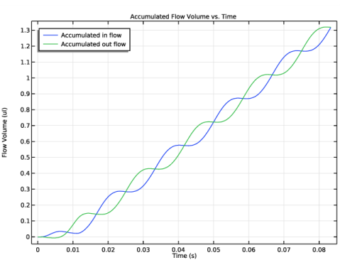
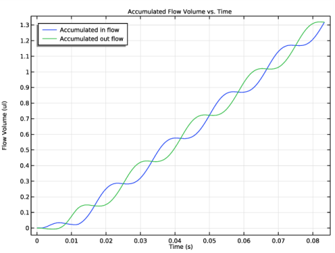
In the Settings window for 1D Plot Group, type Accumulated Flow Volume vs. Time in the Label text field.
2
Click to expand the Title section. From the Title type list, choose Label.
3
Locate the Plot Settings section. Select the y-axis label check box.
4
5
Locate the Legend section. From the Position list, choose Upper left.
Global 1
1
In the Model Builder window, expand the Accumulated Flow Volume vs. Time node, then click Global 1.
2
In the Settings window for Global, locate the y-Axis Data section.
3
4
In the Accumulated Flow Volume vs. Time toolbar, click  Plot.
We see that the in flow and out flow are staggered as one would expect from how the pump works. This can also be seen in the flow rate as a function of time. The volume conservation is shown by plotting the sum of the flow rates and the rate of volume change by the deflection of the membrane.
Flow Rate vs. Time & Volume Conservation
1
In the Model Builder window, right-click Accumulated Flow Volume vs. Time and choose Duplicate.
2
In the Model Builder window, click Accumulated Flow Volume vs. Time 1.
3
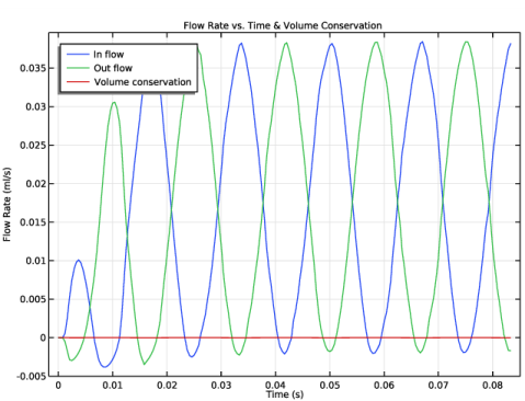
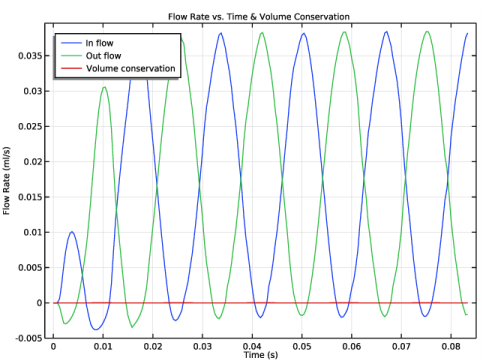
In the Settings window for 1D Plot Group, type Flow Rate vs. Time & Volume Conservation in the Label text field.
4
Locate the Plot Settings section. In the y-axis label text field, type Flow Rate (ml/s).
Global 1
1
In the Model Builder window, click Global 1.
2
In the Settings window for Global, locate the y-Axis Data section.
3
4
In the Flow Rate vs. Time & Volume Conservation toolbar, click  Plot.
The sum of the rates is zero, confirming the volume conservation. Now create a plot of the velocity field showing the fluid and solid movement on the symmetry plane.
Velocity Field
1
In the Home toolbar, click  Add Plot Group and choose 3D Plot Group.
2
In the Settings window for 3D Plot Group, type Velocity Field in the Label text field.
3
Click to expand the Title section. From the Title type list, choose Label.
Surface 1
1
Right-click Velocity Field and choose Surface.
2
In the Settings window for Surface, locate the Expression section.
3
In the Expression text field, type log10(spf.U/1[mm/s]).
Selection 1
1
Right-click Surface 1 and choose Selection.
2
In the Settings window for Selection, locate the Selection section.
3
From the Selection list, choose Box 4 - Symmetry Plane.
Surface 2
1
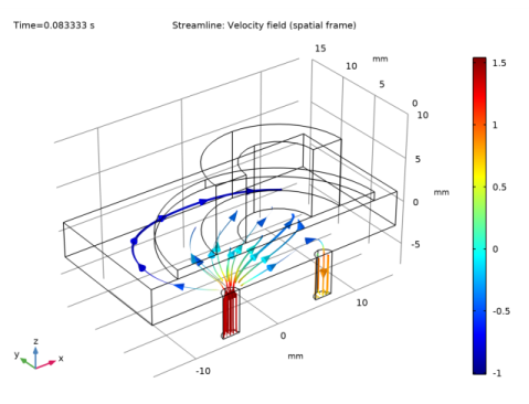
In the Model Builder window, under Results>Velocity Field right-click Surface 1 and choose Duplicate.
2
In the Settings window for Surface, locate the Expression section.
3
In the Expression text field, type log10(solid.vel/1[mm/s]).
4
Click to expand the Inherit Style section. From the Plot list, choose Surface 1.
Arrow Surface 1
1
In the Model Builder window, right-click Velocity Field and choose Arrow Surface.
2
In the Settings window for Arrow Surface, locate the Expression section.
3
In the x component text field, type u2.
4
In the y component text field, type v2.
5
In the z component text field, type w2.
6
Locate the Coloring and Style section. From the Arrow length list, choose Normalized.
7
From the Color list, choose White.
Selection 1
1
Right-click Arrow Surface 1 and choose Selection.
2
In the Settings window for Selection, locate the Selection section.
3
From the Selection list, choose Box 4 - Symmetry Plane.
Arrow Surface 2
1
In the Model Builder window, under Results>Velocity Field right-click Arrow Surface 1 and choose Duplicate.
2
In the Settings window for Arrow Surface, locate the Expression section.
3
In the x component text field, type ut.
4
In the y component text field, type vt.
5
In the z component text field, type wt.
6
In the Velocity Field toolbar, click  Plot.
7
Click the  Go to XZ View button in the Graphics toolbar.
This shows a time point when the fluid is being drawn in through the inlet. Take a look at a different time point when the fluid is being pushed out through the outlet.
Velocity Field
1
In the Model Builder window, click Velocity Field.
2
In the Settings window for 3D Plot Group, locate the Data section.
3
From the Time (s) list, choose 0.075.
4
In the Velocity Field toolbar, click  Plot.
Create streamline plots for the same two time points.
Fluid Streamlines
1
In the Home toolbar, click  Add Plot Group and choose 3D Plot Group.
2
In the Settings window for 3D Plot Group, type Fluid Streamlines in the Label text field.
Streamline 1
1
Right-click Fluid Streamlines and choose Streamline.
2
In the Settings window for Streamline, locate the Expression section.
3
In the x component text field, type u2.
4
In the y component text field, type v2.
5
In the z component text field, type w2.
Color Expression 1
1
Right-click Streamline 1 and choose Color Expression.
2
In the Settings window for Color Expression, locate the Expression section.
3
In the Expression text field, type log10(spf.U/1[mm/s]).
Streamline 1
1
In the Model Builder window, click Streamline 1.
2
In the Settings window for Streamline, locate the Selection section.
3
From the Selection list, choose Union 1 - Inlet and Outlet.
4
Locate the Coloring and Style section. Find the Line style subsection. From the Type list, choose Ribbon.
5
Find the Point style subsection. From the Type list, choose Arrow.
6
In the Fluid Streamlines toolbar, click  Plot.
7
Click the  Go to Default View button in the Graphics toolbar.
This shows a time point when the fluid is being drawn in through the inlet. Take a look at a different time point when the fluid is being pushed out through the outlet.
Fluid Streamlines
1
In the Model Builder window, click Fluid Streamlines.
2
In the Settings window for 3D Plot Group, locate the Data section.
3
From the Time (s) list, choose 0.075.
4
In the Fluid Streamlines toolbar, click  Plot.