|
|
|
|
•
|
|
•
|
|
•
|
Ground (0 dof)
|
|
•
|
|
•
|
|
•
|
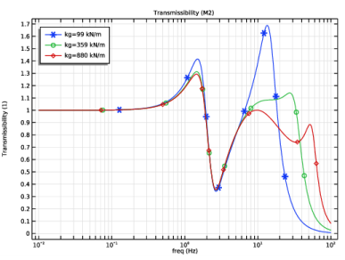
Soft soil (99 kN/m)
|
|
•
|
Hard soil (359 kN/m)
|
|
•
|
Very hard soil (880 kN/m)
|
|
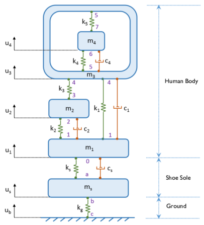
6.15 kg
|
||
|
6 kg
|
||
|
12.58 kg
|
||
|
50.34 kg
|
||
|
6 kN/m
|
||
|
6 kN/m
|
||
|
10 kN/m
|
||
|
10 kN/m
|
||
|
18 kN/m
|
||
|
0.3 kN-s/m
|
||
|
0.65 kN-s/m
|
||
|
1.9 kN-s/m
|
||
|
0.3 kg
|
||
|
403 kN/m
|
||
|
2170 kN-s/m
|
||
|
880 kN/m
|
||
|
10 mm
|
|
•
|
Fixed Node is the default node in the Lumped Mechanical System interface. It can be disabled if none of the nodes of the system are fixed.
|
|
•
|
Lumped models in general have very few degrees of freedom compared to FEM models. Thus, for the eigenfrequency computation, All (filled matrix) can be used in Eigenfrequency search method.
|
|
•
|
Default plots from the Lumped Mechanical System interface can be customized by selecting the appropriate options in the Results section of various features.
|
|
1
|
|
2
|
|
3
|
Click Add.
|
|
4
|
Click
|
|
5
|
|
6
|
Click
|
|
1
|
|
2
|
|
3
|
|
4
|
Browse to the model’s Application Libraries folder and double-click the file lumped_human_body_parameters.txt.
|
|
1
|
|
2
|
Right-click Component 1 (comp1)>Lumped Mechanical System (lms)>Fixed Node 1 (fix1) and choose Disable.
|
|
1
|
|
2
|
|
4
|
|
5
|
Locate the Results section. Find the Add the following to default results subsection. Clear the Force check box.
|
|
1
|
|
2
|
|
4
|
|
5
|
Locate the Results section. Find the Add the following to default results subsection. Clear the Displacement check box.
|
|
1
|
|
2
|
|
4
|
|
5
|
Locate the Results section. Find the Add the following to default results subsection. Clear the Force check box.
|
|
6
|
Clear the Displacement check box.
|
|
1
|
|
2
|
|
4
|
|
5
|
Locate the Results section. Find the Add the following to default results subsection. Clear the Force check box.
|
|
1
|
|
2
|
|
4
|
|
5
|
Locate the Results section. Find the Add the following to default results subsection. Clear the Displacement check box.
|
|
1
|
|
2
|
|
4
|
|
5
|
Locate the Results section. Find the Add the following to default results subsection. Clear the Force check box.
|
|
1
|
|
2
|
|
4
|
|
5
|
Locate the Results section. Find the Add the following to default results subsection. Clear the Displacement check box.
|
|
1
|
|
2
|
|
3
|
|
4
|
|
5
|
Locate the Results section. Find the Add the following to default results subsection. Clear the Force check box.
|
|
6
|
Clear the Displacement check box.
|
|
1
|
|
2
|
|
4
|
|
5
|
Locate the Results section. Find the Add the following to default results subsection. Clear the Force check box.
|
|
1
|
|
2
|
|
4
|
|
5
|
Locate the Results section. Find the Add the following to default results subsection. Clear the Displacement check box.
|
|
1
|
|
2
|
|
3
|
|
4
|
|
5
|
Locate the Results section. Find the Add the following to default results subsection. Clear the Displacement check box.
|
|
1
|
|
2
|
|
3
|
|
4
|
|
5
|
Locate the Results section. Find the Add the following to default results subsection. Clear the Force check box.
|
|
6
|
Clear the Displacement check box.
|
|
1
|
|
2
|
|
3
|
|
4
|
|
5
|
Locate the Results section. Find the Add the following to default results subsection. Clear the Force check box.
|
|
1
|
|
2
|
|
3
|
|
4
|
|
5
|
Locate the Results section. Find the Add the following to default results subsection. Clear the Force check box.
|
|
6
|
Clear the Displacement check box.
|
|
1
|
|
2
|
|
4
|
|
1
|
|
2
|
|
3
|
|
4
|
|
1
|
|
2
|
|
3
|
|
4
|
|
5
|
|
1
|
|
2
|
|
3
|
Click
|
|
1
|
|
2
|
|
3
|
|
4
|
|
1
|
|
2
|
|
3
|
|
4
|
|
5
|
|
6
|
|
1
|
|
2
|
|
3
|
|
4
|
|
5
|
|
6
|
|
7
|
|
1
|
|
2
|
|
3
|
|
4
|
|
5
|
|
6
|
|
7
|
|
1
|
|
2
|
|
3
|
|
4
|
|
5
|
|
6
|
|
7
|
|
1
|
|
2
|
|
3
|
|
4
|
|
5
|
|
1
|
|
2
|
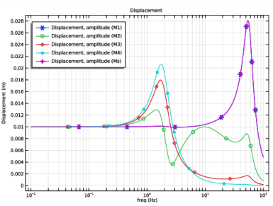
In the Settings window for Global, click Replace Expression in the upper-right corner of the y-Axis Data section. From the menu, choose Component 1 (comp1)>Lumped Mechanical System>Two port components>M2>lms.M2_uAmp - Displacement, amplitude (M2) - m.
|
|
3
|
|
4
|
Click to expand the Coloring and Style section. Find the Line markers subsection. From the Marker list, choose Cycle.
|
|
5
|
|
6
|
|
7
|