PDF

High-Cycle Fatigue of a Reciprocating Piston Engine
Introduction
In a reciprocating piston engine, the connecting rods transfer rotating motion into reciprocating motion. The connecting rods are constantly subjected to high stresses and the load increases with the engine speed. A failure of one part in the engine usually results in a replacement of the whole engine. It is therefore of crucial importance to design all engine parts so that none of them fail during the operational lifetime. The connecting rods are identified as critical parts and are here analyzed from the fatigue perspective. The fatigue lifetime is predicted using the Basquin high-cycle fatigue criterion.
This example is based on the model Three-Cylinder Reciprocating Engine, where one connecting rod is modeled as a flexible body while the remaining parts are modeled as rigid bodies. The connections between the different parts are obtained by using a different type of joints. This technique significantly reduces the model size while maintaining the force equilibrium in the assembly.
Model Definition
The three-cylinder engine is presented in Figure 1, and it operates at 1000 RPM. Its material data is taken from structural steel. Additional information regarding its set up can be found in the documentation for Three-Cylinder Reciprocating Engine.
The material data from fatigue tests is summarized in Figure 2. A Basquin relation with the material constants σf' = 1043 MPa and b = 0.116 gives a good fit to the experimental results. The material exhibits a fatigue limit at 210 MPa.
Figure 1: Geometry of the reciprocating piston engine.
Figure 2: Fatigue material curve.
Results and Discussion
At first, stresses in a fillet of the piston end of the connecting rod are examined, see Figure 3. A fillet is chosen since a stress concentration due to geometrical change is expected there. A few revolutions must be computed before a steady state behavior is obtained. From cycle three, the stress history for each consecutive cycles seems to repeat itself. Both the peak stress and the of the stress cycle in general is about the same. The stress history is dominated by the third principal stress since the connecting rod is in compression. The two other principal stresses are small so that the stress state at the fillet can be considered uniaxial. Therefore the third principal stress is taken as the amplitude stress in the Basquin relation as opposed to the von Mises stress which may be more appropriate in a multiaxial loading. The fatigue life prediction is shown in Figure 4.
Figure 3: Stress history in the connecting rod.
Figure 4: Fatigue life prediction in the connecting rod.
The critical point is at the fillet close to the top end of the connecting rod where the Basquin model predicts a fatigue life which is longer than ten billion (10·109) cycles. This is an extremely long life. It can therefore be expected that the stress in the assembly is below the endurance limit that for the used material is 210 MPa. By using the Basquin relation
where σa is the stress amplitude and N is the number of cycles to failure, the fatigue endurance limit life can be back-calculated to 120 million cycles. This is less than the calculated value, see Figure 4, and therefore the connecting rod is designed for infinite life. This could have been already observed in Figure 3 where the stress history is shown. Since the principal stress range is about 110 MPa the stress amplitude is about 55 MPa and that is below the endurance limit of the material.
Notes About the COMSOL Implementation
In the Basquin evaluation the parameter Cycle cutoff can be used to incorporate the effect of endurance limit. The number of cycles that gives the endurance limit must then be back-calculated.
Application Library path: Multibody_Dynamics_Module/Automotive_and_Aerospace/engine_fatigue
Modeling Instructions
Root
In this example you will start from an existing model from the Multibody Dynamics Module.
1
From the File menu, choose Open.
2
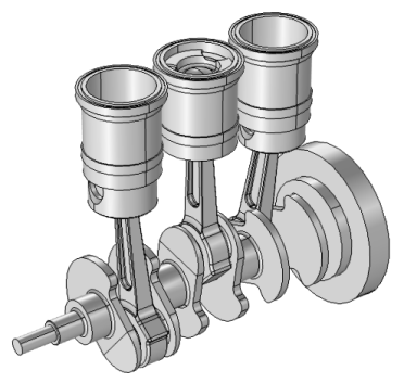
From the Application Libraries root, browse to the folder Multibody_Dynamics_Module/Automotive_and_Aerospace and double-click the file reciprocating_engine.mph.
If the model was stored without solutions, you will now have to run the two existing studies before continuing. To run the Study: Thermodynamic analysis, you need to enable the Pressure Work node by right clicking on Component 1 > Heat Transfer in Fluids > Fluid 1 > Pressure Work 1 and then clicking Enable. This may require extra license.
Evaluate how stresses develop. Examine one point in a fillet close to the small end of the connecting rod.
Results
Stress history: Connecting rod
1
In the Home toolbar, click  Add Plot Group and choose 1D Plot Group.
2
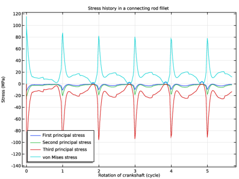
In the Settings window for 1D Plot Group, type Stress history: Connecting rod in the Label text field.
3
Locate the Data section. From the Dataset list, choose Study: Multibody Analysis/Solution 2 (3) (sol2).
Point Graph 1
1
Right-click Stress history: Connecting rod and choose Point Graph.
2
In the Settings window for Point Graph, locate the Selection section.
3
Click  Paste Selection.
4
In the Paste Selection dialog box, type 834 in the Selection text field.
5
6
In the Settings window for Point Graph, locate the y-Axis Data section.
7
In the Expression text field, type mbd.sp1.
8
From the Unit list, choose MPa.
9
Locate the x-Axis Data section. From the Parameter list, choose Expression.
10
In the Expression text field, type theta/(2*pi).
11
Click to expand the Legends section. Select the Show legends check box.
12
From the Legends list, choose Manual.
13
14
In the Stress history: Connecting rod toolbar, click  Plot.
Point Graph 2
1
Right-click Point Graph 1 and choose Duplicate.
2
In the Settings window for Point Graph, locate the y-Axis Data section.
3
In the Expression text field, type mbd.sp2.
4
Locate the Legends section. In the table, enter the following settings:
5
In the Stress history: Connecting rod toolbar, click  Plot.
Point Graph 3
1
Right-click Point Graph 2 and choose Duplicate.
2
In the Settings window for Point Graph, locate the y-Axis Data section.
3
In the Expression text field, type mbd.sp3.
4
Locate the Legends section. In the table, enter the following settings:
5
In the Stress history: Connecting rod toolbar, click  Plot.
Point Graph 4
1
Right-click Point Graph 3 and choose Duplicate.
2
In the Settings window for Point Graph, locate the y-Axis Data section.
3
In the Expression text field, type mbd.mises.
4
Locate the Legends section. In the table, enter the following settings:
5
In the Stress history: Connecting rod toolbar, click  Plot.
Stress history: Connecting rod
1
In the Model Builder window, click Stress history: Connecting rod.
2
In the Settings window for 1D Plot Group, locate the Plot Settings section.
3
Select the x-axis label check box.
4
In the associated text field, type Rotation of crankshaft (cycle).
5
Select the y-axis label check box.
6
7
Click to expand the Title section. From the Title type list, choose Manual.
8
In the Title text area, type Stress history in a connecting rod fillet.
9
Locate the Legend section. From the Position list, choose Lower left.
10
In the Stress history: Connecting rod toolbar, click  Plot.
Add Physics
1
In the Home toolbar, click  Add Physics to open the Add Physics window.
2
Go to the Add Physics window.
3
In the tree, select Structural Mechanics>Fatigue (ftg).
4
Find the Physics interfaces in study subsection. In the table, clear the Solve check boxes for Study: Thermodynamic Analysis and Study: Multibody Analysis.
5
Click Add to Multibody Analysis in the window toolbar.
6
In the Home toolbar, click  Add Physics to close the Add Physics window.
Fatigue (ftg)
Stress-Life 1
1
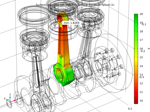
Right-click Multibody Analysis (comp2)>Fatigue (ftg) and choose the boundary evaluation Stress-Life.
Select boundaries of the connecting rod in the middle. It is easier to do using a boundary selection from domain.
Definitions (comp2)
Middle Rod Boundaries
1
In the Model Builder window, expand the Multibody Analysis (comp2)>Definitions node.
2
Right-click Multibody Analysis (comp2)>Definitions>Selections and choose Explicit.
3
In the Settings window for Explicit, type Middle Rod Boundaries in the Label text field.
4
5
Locate the Output Entities section. From the Output entities list, choose Adjacent boundaries.
Fatigue (ftg)
Stress-Life 1
1
In the Model Builder window, under Multibody Analysis (comp2)>Fatigue (ftg) click Stress-Life 1.
2
In the Settings window for Stress-Life, locate the Boundary Selection section.
3
From the Selection list, choose Middle Rod Boundaries.
4
Locate the Fatigue Model Selection section. From the Criterion list, choose Basquin.
5
Locate the Solution Field section. From the Physics interface list, choose Multibody Dynamics (mbd).
6
Locate the Fatigue Model Parameters section. From the σf list, choose User defined. In the associated text field, type 1.043e9.
7
From the b list, choose User defined. In the associated text field, type -0.116.
The cutoff value can be used to specify the endurance limit. In this example the cutoff is set to a high value in order to examine how the Basquin model predicts lifetime in case the material did not have an endurance limit.
8
Locate the Evaluation Settings section. In the Ncut text field, type 1e20.
Root
In the Home toolbar, click  Windows and choose Add Study.
Add Study
1
Go to the Add Study window.
2
Find the Studies subsection. In the Select Study tree, select Preset Studies for Selected Physics Interfaces>Fatigue>Fatigue.
3
Click Add Study in the window toolbar.
Study 3
Step 1: Fatigue
1
In the Settings window for Fatigue, locate the Study Settings section.
2
Select the Include geometric nonlinearity check box.
3
Click to expand the Values of Dependent Variables section. Find the Values of variables not solved for subsection. From the Settings list, choose User controlled.
4
From the Method list, choose Solution.
5
From the Study list, choose Study: Multibody Analysis, Time Dependent.
6
From the Time (s) list, choose From list.
7
In the Time (s) list, choose 0.1368 s, 0.1372 s, 0.1376 s, 0.138 s, 0.1384 s, 0.1388 s, 0.1392 s, 0.1396 s, 0.14 s, 0.1404 s, 0.1408 s, 0.1412 s, 0.1416 s, 0.142 s, 0.1424 s, 0.1428 s, 0.1432 s, 0.1436 s, 0.144 s, 0.1444 s, 0.1448 s, 0.1452 s, 0.1456 s, 0.146 s, 0.1464 s, 0.1468 s, 0.1472 s, 0.1476 s, 0.148 s, 0.1484 s, 0.1488 s, 0.1492 s, 0.1496 s, 0.15 s, 0.1504 s, 0.1508 s, 0.1512 s, 0.1516 s, 0.152 s, 0.1524 s, 0.1528 s, 0.1532 s, 0.1536 s, 0.154 s, 0.1544 s, 0.1548 s, 0.1552 s, 0.1556 s, 0.156 s, 0.1564 s, 0.1568 s, 0.1572 s, 0.1576 s, 0.158 s, 0.1584 s, 0.1588 s, 0.1592 s, 0.1596 s, and 0.16 s.
8
In the Model Builder window, click Study 3.
9
In the Settings window for Study, type Study: Fatigue analysis in the Label text field.
10
In the Home toolbar, click  Compute.
Results
Cycles to Failure (ftg)
The plot showing cycles to failure (Figure 4) is created by default.