PDF

Spring-Loaded Centrifugal Governor
Introduction
A centrifugal governor is a device used for controlling the angular speed of rotating machinery. One of the most common applications of centrifugal governors is to control the RPM of an engine by regulating the fuel supply. Power is transferred to the governor through the output shaft of the engine. As the RPM of the engine increase, the governor throttles the fuel supply, thus decreasing the energy input to the engine.
Model Definition
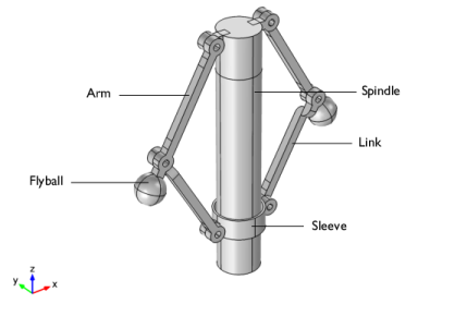
This model demonstrates the modeling of a spring loaded centrifugal governor. The centrifugal governor (Figure 1) consists of a spindle, two arms, two links, two flyballs, and a sleeve. The spindle is connected to the output shaft of the engine. The arms are connected to the spindle through hinge joints at one end, and flyballs are attached to the other end.
Figure 1: Geometry of the centrifugal governor.
Each link is connected to the respective arm and to the sleeve through hinge joints. The sleeve is mounted over the spindle and is free to slide. This is modeled with a prismatic joint. The hinge joint has one rotational degree of freedom, whereas the prismatic joint has one translational degree of freedom along the spindle axis.
In this model, a spring is connected between the sleeve and the spindle to restrict the sleeve’s sliding motion. To stabilize the sleeve at its equilibrium position, a dashpot is attached between the sleeve and the spindle. The spring and the dashpot are available to prismatic joints.
As the spindle rotates with a constant RPM, the centrifugal force makes the arms, links, and flyballs move outward, causing the sleeve to slide on the spindle and move upward.
The spring attached to the sleeve restricts the outward motion, making the sleeve oscillate around an equilibrium position where the net force is zero. This oscillation, caused by inertial effects, is dampened by the dashpot.
The equilibrium position of the sleeve is governed by the RPM of the spindle. Once the RPM of the spindle is increased, the sleeve moves to a new equilibrium position.
Results and Discussion
Figure 2: Displacement of various parts of the centrifugal governor. Trajectory of one of the flyballs is also shown.
Figure 2 displays the total displacement of all the parts and the trajectory of one of the flyballs at a particular moment. The maximum displacement that can be seen in the flyballs, is the combination of rotational motion and outward motion.
Figure 3 displays the stress generated in the governor components at a particular moment during the operation. The stresses are maximum in the arms and links, and they are concentrated near the joints.
Figure 3: von Mises stress in the centrifugal governor. Trajectory of one of the flyballs is also shown.
Figure 4 depicts the displacement of the sleeve with respect to the spindle during operation. The displacement is plotted against the number of revolutions of the spindle. This figure shows how the sleeve moves to an equilibrium position from the initial state. After a few revolutions of the spindle, RPM is gradually doubled and as a result the sleeve moves to a new equilibrium position.
Figure 5 shows the phase portrait of the sleeve’s sliding motion. The phase portrait gives more insight about the motion and clearly shows the two equilibrium positions corresponding to the two different RPM values.
Figure 4: Relative displacement of the sleeve with respect to the spindle.
Figure 5: Phase portrait of the sleeve’s sliding motion.
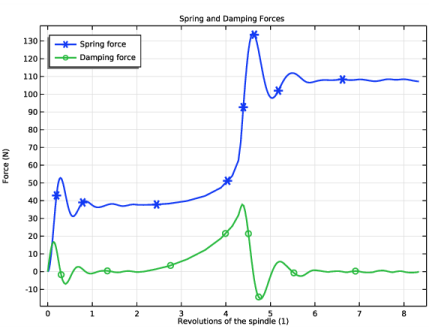
The spring and damping forces attached to the sleeve-spindle joint are shown in Figure 6. These forces balance the external force applied on the sleeve due to the centrifugal force on the other governor’s parts. It is clear that these forces vary significantly whenever there is a change in speed. The damping force goes to zero whereas the spring force resists the external force.
Figure 6: Spring and damping force in the spring-dashpot attached between the sleeve and the spindle.
Figure 7 shows the spatial components of the force in the spindle-arm hinge joint. The x and y components have an oscillatory nature and are shifted relatively to each other by a quarter of a revolution. The z component of the force goes toward a constant value controlled by the RPM. Also, the amplitude of both the x and y components changes once the RPM value changes. This demonstrates the change in the force equilibrium of the system.
Figure 7: Forces in the hinge joint between the spindle and the arm.
Notes About the COMSOL Implementation
Application Library path: Multibody_Dynamics_Module/Automotive_and_Aerospace/centrifugal_governor
Modeling Instructions
From the File menu, choose New.
New
In the New window, click  Model Wizard.
Model Wizard
1
In the Model Wizard window, click  3D.
2
In the Select Physics tree, select Structural Mechanics>Multibody Dynamics (mbd).
3
Click Add.
4
Click  Study.
5
In the Select Study tree, select General Studies>Time Dependent.
6
Geometry 1
Import 1 (imp1)
1
In the Home toolbar, click  Import.
2
In the Settings window for Import, locate the Import section.
3
Click Browse.
4
5
Click Import.
Form Union (fin)
1
In the Model Builder window, under Component 1 (comp1)>Geometry 1 click Form Union (fin).
2
In the Settings window for Form Union/Assembly, locate the Form Union/Assembly section.
3
From the Action list, choose Form an assembly.
4
Clear the Create pairs check box.
5
Click  Build Selected.
Definitions
Variables 1
1
In the Home toolbar, click  Variables and choose Local Variables.
2
In the Settings window for Variables, locate the Variables section.
3
Use a step function to increase the RPM of the spindle.
Step 1 (step1)
1
In the Home toolbar, click  Functions and choose Local>Step.
2
In the Settings window for Step, locate the Parameters section.
3
In the Location text field, type 0.125.
4
In the From text field, type 1.
5
In the To text field, type 2.
6
Click to expand the Smoothing section. In the Size of transition zone text field, type 0.01.
Add Material
1
In the Home toolbar, click  Add Material to open the Add Material window.
2
Go to the Add Material window.
3
In the tree, select Built-in>Structural steel.
4
Click Add to Component in the window toolbar.
5
In the Home toolbar, click  Add Material to close the Add Material window.
Multibody Dynamics (mbd)
To avoid transient effects, the governor is initialized to rotate about the z-axis.
1
In the Model Builder window, under Component 1 (comp1) click Multibody Dynamics (mbd).
2
In the Settings window for Multibody Dynamics, click to expand the Initial Values section.
3
Specify the ω vector as
Attachment 1
1
In the Physics toolbar, click  Boundaries and choose Attachment.
2
Attachments
You can create the remaining attachments using the information given in the table below:
Prismatic Joint 1
1
In the Physics toolbar, click  Global and choose Prismatic Joint.
2
In the Settings window for Prismatic Joint, locate the Attachment Selection section.
3
From the Source list, choose Attachment 1.
4
From the Destination list, choose Attachment 2.
5
Locate the Axis of Joint section. Specify the e0 vector as
Spring and Damper 1
1
In the Physics toolbar, click  Attributes and choose Spring and Damper.
2
In the Settings window for Spring and Damper, locate the Spring and Damper: Translational section.
3
In the ku text field, type k.
4
In the cu text field, type c.
Hinge Joint 1
1
In the Physics toolbar, click  Global and choose Hinge Joint.
2
In the Settings window for Hinge Joint, locate the Attachment Selection section.
3
From the Source list, choose Attachment 3.
4
From the Destination list, choose Attachment 4.
5
Locate the Axis of Joint section. Specify the e0 vector as
Hinge Joint 2
1
Right-click Hinge Joint 1 and choose Duplicate.
2
In the Settings window for Hinge Joint, locate the Attachment Selection section.
3
From the Source list, choose Attachment 5.
4
From the Destination list, choose Attachment 6.
Hinge Joint 3
1
Right-click Hinge Joint 2 and choose Duplicate.
2
In the Settings window for Hinge Joint, locate the Attachment Selection section.
3
From the Source list, choose Attachment 7.
4
From the Destination list, choose Attachment 8.
Hinge Joint 4
1
Right-click Hinge Joint 3 and choose Duplicate.
2
In the Settings window for Hinge Joint, locate the Attachment Selection section.
3
From the Source list, choose Attachment 9.
4
From the Destination list, choose Attachment 10.
Hinge Joint 5
1
Right-click Hinge Joint 4 and choose Duplicate.
2
In the Settings window for Hinge Joint, locate the Attachment Selection section.
3
From the Source list, choose Attachment 11.
4
From the Destination list, choose Attachment 12.
Hinge Joint 6
1
Right-click Hinge Joint 5 and choose Duplicate.
2
In the Settings window for Hinge Joint, locate the Attachment Selection section.
3
From the Source list, choose Attachment 13.
4
From the Destination list, choose Attachment 14.
Use a Hinge Joint node with a Prescribed Motion subnode to model the rotation of the spindle.
Hinge Joint 7
1
Right-click Hinge Joint 6 and choose Duplicate.
2
In the Settings window for Hinge Joint, locate the Attachment Selection section.
3
From the Source list, choose Fixed.
4
From the Destination list, choose Attachment 1.
5
Locate the Axis of Joint section. Specify the e0 vector as
Prescribed Motion 1
1
In the Physics toolbar, click  Attributes and choose Prescribed Motion.
2
In the Settings window for Prescribed Motion, locate the Prescribed Rotational Motion section.
3
From the Prescribed motion through list, choose Angular velocity.
4
In the ωp text field, type omega.
Mesh 1
1
In the Model Builder window, under Component 1 (comp1) click Mesh 1.
2
In the Settings window for Mesh, locate the Physics-Controlled Mesh section.
3
From the Element size list, choose Coarse.
Use a finer mesh to get a more accurate solution.
Study 1
Step 1: Time Dependent
1
In the Model Builder window, under Study 1 click Step 1: Time Dependent.
2
In the Settings window for Time Dependent, locate the Study Settings section.
3
In the Output times text field, type range(0,0.001,0.25).
4
From the Tolerance list, choose User controlled.
5
In the Relative tolerance text field, type 0.001.
Solution 1 (sol1)
1
In the Study toolbar, click  Show Default Solver.
2
In the Model Builder window, expand the Solution 1 (sol1) node, then click Time-Dependent Solver 1.
3
In the Settings window for Time-Dependent Solver, click to expand the Absolute Tolerance section.
4
From the Tolerance method list, choose Manual.
5
Click to expand the Time Stepping section. From the Steps taken by solver list, choose Free.
6
From the Maximum step constraint list, choose Constant.
7
In the Maximum step text field, type 0.005.
Switching off the consistent initialization helps the simulation to start more smoothly. This also avoids high initial forces due to inconsistent initial values.
8
Click to expand the Advanced section. Locate the Time Stepping section. Find the Algebraic variable settings subsection. From the Consistent initialization list, choose Off.
9
In the Study toolbar, click  Compute.
Results
Follow these instructions to generate the displacement plot shown in Figure 2:
Displacement (mbd)
1
In the Model Builder window, under Results click Displacement (mbd).
2
In the Settings window for 3D Plot Group, locate the Data section.
3
From the Time (s) list, choose 0.16.
Point Trajectories 1
1
In the Displacement (mbd) toolbar, click  More Plots and choose Point Trajectories.
2
3
In the Settings window for Point Trajectories, locate the Coloring and Style section.
4
Find the Line style subsection. From the Type list, choose Tube.
Color Expression 1
1
Right-click Point Trajectories 1 and choose Color Expression.
2
In the Settings window for Color Expression, locate the Expression section.
3
In the Expression text field, type t.
4
Locate the Coloring and Style section. Clear the Color legend check box.
Displacement (mbd)
1
Click the  Zoom Extents button in the Graphics toolbar.
2
In the Model Builder window, click Displacement (mbd).
3
In the Displacement (mbd) toolbar, click  Plot.
Follow these instructions to generate the stress plot shown in Figure 3:
Stress
1
Right-click Displacement (mbd) and choose Duplicate.
2
In the Settings window for 3D Plot Group, type Stress in the Label text field.
Surface
1
In the Model Builder window, expand the Stress node, then click Surface.
2
In the Settings window for Surface, click Replace Expression in the upper-right corner of the Expression section. From the menu, choose Component 1 (comp1)>Multibody Dynamics>Stress>mbd.mises - von Mises stress - N/m².
3
In the Stress toolbar, click  Plot.
Use the following instructions to generate a plot for the relative displacement of the sleeve as given in Figure 4:
Relative Displacement
1
In the Home toolbar, click  Add Plot Group and choose 1D Plot Group.
2
In the Settings window for 1D Plot Group, type Relative Displacement in the Label text field.
3
Click to expand the Title section. From the Title type list, choose Label.
Global 1
1
Right-click Relative Displacement and choose Global.
2
In the Settings window for Global, click Replace Expression in the upper-right corner of the y-Axis Data section. From the menu, choose Component 1 (comp1)>Multibody Dynamics>Prismatic joints>Prismatic Joint 1>mbd.prj1.u - Relative displacement - m.
3
Click to expand the Title section. From the Title type list, choose None.
4
Click to expand the Legends section. Clear the Show legends check box.
5
Click to expand the Coloring and Style section. In the Width text field, type 2.
6
Locate the x-Axis Data section. From the Parameter list, choose Expression.
7
In the Expression text field, type N.
Relative Displacement
1
In the Model Builder window, click Relative Displacement.
2
In the Relative Displacement toolbar, click  Plot.
Use the following instructions to generate a phase portrait of the sleeve motion as given in Figure 5:
Phase Portrait
1
In the Home toolbar, click  Add Plot Group and choose 1D Plot Group.
2
In the Settings window for 1D Plot Group, type Phase Portrait in the Label text field.
3
Locate the Title section. From the Title type list, choose Label.
Global 1
1
Right-click Phase Portrait and choose Global.
2
In the Settings window for Global, click Replace Expression in the upper-right corner of the y-Axis Data section. From the menu, choose Component 1 (comp1)>Multibody Dynamics>Prismatic joints>Prismatic Joint 1>mbd.prj1.u_t - Relative velocity - m/s.
3
Locate the Title section. From the Title type list, choose Manual.
4
In the Title text area, type Phase portrait.
5
Locate the Legends section. Clear the Show legends check box.
6
Locate the Coloring and Style section. In the Width text field, type 2.
7
Locate the x-Axis Data section. From the Parameter list, choose Expression.
8
In the Expression text field, type mbd.prj1.u.
Phase Portrait
1
In the Model Builder window, click Phase Portrait.
2
In the Phase Portrait toolbar, click  Plot.
Follow these instructions to generate a plot for the spring and damping forces as given in Figure 6:
Spring and Damping Forces
1
In the Home toolbar, click  Add Plot Group and choose 1D Plot Group.
2
In the Settings window for 1D Plot Group, type Spring and Damping Forces in the Label text field.
3
Locate the Plot Settings section. Select the y-axis label check box.
4
5
Locate the Title section. From the Title type list, choose Label.
6
Locate the Legend section. From the Position list, choose Upper left.
Global 1
1
Right-click Spring and Damping Forces and choose Global.
2
In the Settings window for Global, locate the y-Axis Data section.
3
4
Locate the x-Axis Data section. From the Parameter list, choose Expression.
5
In the Expression text field, type N.
6
Locate the Coloring and Style section. In the Width text field, type 2.
7
Find the Line markers subsection. From the Marker list, choose Cycle.
8
In the Spring and Damping Forces toolbar, click  Plot.
Follow these instructions to generate a plot of the forces in the joint between the spindle and the arm, as shown in Figure 7:
Joint Forces
1
In the Home toolbar, click  Add Plot Group and choose 1D Plot Group.
2
In the Settings window for 1D Plot Group, type Joint Forces in the Label text field.
3
Locate the Title section. From the Title type list, choose Label.
4
Locate the Plot Settings section. Select the y-axis label check box.
5
6
Locate the Legend section. From the Position list, choose Upper left.
Global 1
1
Right-click Joint Forces and choose Global.
2
In the Settings window for Global, click Replace Expression in the upper-right corner of the y-Axis Data section. From the menu, choose Component 1 (comp1)>Multibody Dynamics>Hinge joints>Hinge Joint 3>Joint force - N>mbd.hgj3.Fx - Joint force, x component.
3
Click Add Expression in the upper-right corner of the y-Axis Data section. From the menu, choose Component 1 (comp1)>Multibody Dynamics>Hinge joints>Hinge Joint 3>Joint force - N>mbd.hgj3.Fy - Joint force, y component.
4
Click Add Expression in the upper-right corner of the y-Axis Data section. From the menu, choose Component 1 (comp1)>Multibody Dynamics>Hinge joints>Hinge Joint 3>Joint force - N>mbd.hgj3.Fz - Joint force, z component.
5
Locate the x-Axis Data section. From the Parameter list, choose Expression.
6
In the Expression text field, type N.
7
Locate the Coloring and Style section. In the Width text field, type 2.
8
Find the Line markers subsection. From the Marker list, choose Cycle.
9
In the Joint Forces toolbar, click  Plot.
Finally, generate an animation of the stress distribution in the centrifugal governor during its operation.
Animation 1
1
In the Results toolbar, click  Animation and choose Player.
2
In the Settings window for Animation, locate the Scene section.
3
From the Subject list, choose Stress.
4
Locate the Frames section. In the Number of frames text field, type 100.
5
Right-click Animation 1 and choose Play.