PDF

Acoustics of a Living Room
Introduction
The sound we experience from our stereo or home theater systems in our living rooms is influenced not only by the quality of loudspeakers, but other factors, for example, the shape of the room, and the type and placement of the furniture. Reflections from walls and windows can both enhance and distort the sound that reaches our ears, and the low bass notes from the speaker woofer units can shake the windows and make the floor vibrate. This happens only for certain frequencies — the eigenfrequencies of the room. The simulation we set-up in this tutorial solves for the eigenfrequencies of a living room in the low frequency range, and analyzes the acoustic field in the room when the sound sources are the woofer units. The analysis is useful, for example, when optimizing for loudspeaker locations inside a living room.
Model Definition
The geometry for the living room used in this analysis is synchronized from Revit® through the LiveLink interface. The room is equipped with a flat-screen TV, a TV stand, a sideboard, a table, two speakers, a bookcase, and two couches. The Revit project file has been saved with the synchronization settings that generate and transfer the volume of the living room, the walls as solid objects, and the furniture. It is not necessary for the analysis to include fully detailed geometry for the furniture in the room. The bookcase is synchronized as a bounding box, while the other furniture items include the original detail level. Further simplifications are done to the synchronized furniture objects inside COMSOL Multiphysics. Selections that are used for model settings are generated for all geometric objects during synchronization.
Figure 1: The room geometry and boundary conditions.
The simulation is set-up with the Pressure Acoustics, Frequency Domain interface to study the sound propagation in free air. Most boundaries in the model — walls, floor, ceiling, and furniture — are assumed to be perfectly rigid (sound hard boundaries), except for the soft surfaces of the two couches. On the couch surfaces an impedance value is set that represents the sound dampening and absorption properties of the material. A normal acceleration is applied to the boundaries that represent the woofer units in the model.
Two studies are added to the model. The eigenfrequency analysis computes the resonance frequencies of the room in the vicinity of 10 Hz together with the corresponding eigenmodes. The frequency domain analysis is set-up to run at 100 Hz.
Results and Discussion
The eigenmodes shows the pressure distribution at the resonance frequencies. Specifically they allow us to identify where there will be no sound (at the nodes) and where the sound will be amplified (at the antinodes). The absolute in an eigenfrequency study do not have any physical meaning.
The real part of the complex valued eigenfrequency represents the frequency at which the system is resonant. The imaginary part is related to the losses at the eigenfrequency an thus the Q-factor of the resonance.
All modes have local maxima in the corners of an empty room so speakers in the corners excite all eigenfrequencies. This simulation predicts eigenmodes that resemble those of the corresponding empty room. The higher the frequency, the more the placing of the furniture matters. The prediction that speakers placed in the corners of the room excite many eigenmodes and give a fuller and more neutral sound, however, holds for real-life rooms.
Figure 2: The sound pressure distribution for an eigenfrequency of 38.4 Hz. The real part of the pressure is visualized as an isosurface plot, and the absolute value of the pressure as a boundary plot.
The results of the frequency domain study allow us to study the acoustic field in the room for the chosen frequency, in this case 100 Hz. More specifically it can be used to extract a transfer function from the speaker to any listening location. This can, for example, be used to fine-tune the phase difference between the speakers to optimize the sound in a specific location of the room.
Figure 3: The sound pressure level produced from the speaker for a frequency of 100 Hz.
Intensity plots, such as the one displayed in Figure 4, allow a visual inspection of the energy flow from the loudspeakers. Typically near resonances the flow will be toward specific points in space.
Figure 4: Streamline plot that visualizes the energy flow from the sound sources at 100 Hz.
Application Library path: LiveLink_for_Revit/Tutorials,_LiveLink_Interface/living_room_acoustics_llrevit
Modeling Instructions
1
In Revit open the file house_living_room.rvt located in the model’s Application Library folder.
2
3
From the File menu, choose New.
New
In the New window, click  Model Wizard.
Model Wizard
1
In the Model Wizard window, click  3D.
2
In the Select Physics tree, select Acoustics>Pressure Acoustics>Pressure Acoustics, Frequency Domain (acpr).
3
Click Add.
4
Click  Study.
5
In the Select Study tree, select General Studies>Frequency Domain.
6
Geometry 1
Make sure that the CAD Import Module kernel is used.
1
In the Model Builder window, under Component 1 (comp1) click Geometry 1.
2
In the Settings window for Geometry, locate the Advanced section.
3
From the Geometry representation list, choose CAD kernel.
LiveLink for Revit 1 (cad1)
1
In the Home toolbar, click  LiveLink and choose LiveLink for Revit.
2
In the Settings window for LiveLink for Revit, locate the Synchronize section.
3
Click Synchronize.
For the synchronization to start a floor plan or section view needs to be active in the Revit software. In case the synchronization does not start switch to Revit, and activate the Level 1 floor plan view. During synchronization the geometry for the living room and the selected elements are generated and transferred to the COMSOL model.
4
Click the  Wireframe Rendering button in the Graphics toolbar.
5
Click to expand the Object Selections section. The synchronized objects are included in automatically generated selections that we will use for setting up the simulation. Clicking on a selection in the table highlights the corresponding objects in the Graphics window.
Room Bounding Solids
Start with creating union selections to be used as inputs to the geometry operations that will create the final geometry for the simulation.
1
In the Geometry toolbar, click  Selections and choose Union Selection.
2
In the Settings window for Union Selection, type Room Bounding Solids in the Label text field.
3
Locate the Geometric Entity Level section. From the Level list, choose Object.
4
Locate the Input Entities section. Click  Add.
5
In the Add dialog box, in the Selections to add list, choose Floors:Generic-12", Roofs:Generic-12", Walls:BasicWall:Generic-8", and Walls:BasicWall:Interior-5"Partition(2-hr).To select several selections from the list hold down Ctrl while clicking the selections.
6
Room
1
In the Geometry toolbar, click  Selections and choose Union Selection.
2
In the Settings window for Union Selection, type Room in the Label text field.
3
Locate the Geometric Entity Level section. From the Level list, choose Object.
4
Locate the Input Entities section. Click  Add.
5
In the Add dialog box, in the Selections to add list, choose Air:Living room 5, Surface:Doors:M_Double-Glass2:1830x2134mm, Surface:Walls:CurtainWall:CurtainWall1, Surface:Windows:M_CasementDblwithTrim:1220x1220mm, Surface:Windows:M_Skylight:0610x0686mm, and Room Bounding Solids.
6
Furniture
1
In the Geometry toolbar, click  Selections and choose Union Selection.
2
In the Settings window for Union Selection, type Furniture in the Label text field.
3
Locate the Geometric Entity Level section. From the Level list, choose Object.
4
Locate the Input Entities section. Click  Add.
5
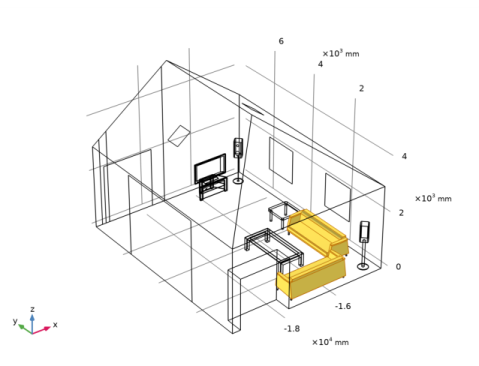
In the Add dialog box, in the Selections to add list, choose Furniture:FloorstandingSpeaker:FloorstandingSpeaker, Furniture:M_Entertainmentcenter:1830x1830x0610mm, Furniture:M_Sofa-Pensi:2134mm, Furniture:M_Table-Coffee:0915x1830x0457mm, Furniture:M_Table-End:0762x0762mm, Furniture:M_TV-FlatScreen:1270mm, and Furniture:M_TVStand:M_TVStand.
6
To be able to use the objects in the defined selections in the model set-up, they need to become part of the final geometry. To incorporate all objects into a single solid object use the Convert to Solid geometry operation.
Convert to Solid 1 (csol1)
1
In the Geometry toolbar, click  Conversions and choose Convert to Solid.
2
In the Settings window for Convert to Solid, locate the Input section.
3
From the Input objects list, choose Room.
4
From the Repair tolerance list, choose Relative.
5
Click  Build All Objects.
Since only the room volume is needed at the end, delete the domains for the walls, roof and floor.
Delete Entities 1 (del1)
1
In the Geometry toolbar, click  Delete.
2
In the Settings window for Delete Entities, locate the Entities or Objects to Delete section.
3
From the Geometric entity level list, choose Domain.
4
From the Selection list, choose Room Bounding Solids.
5
Click  Build All Objects.
Difference 1 (dif1)
To obtaining the computational volume subtract the objects for the furniture from the object for the room.
1
In the Geometry toolbar, click  Booleans and Partitions and choose Difference.
2
In the Settings window for Difference, locate the Difference section.
3
From the Objects to add list, choose Room.
4
From the Objects to subtract list, choose Furniture.
5
Click  Build Selected.
Now use the defeaturing tools to find and remove small details from the geometry of the furniture.
6
In the Geometry toolbar, click  Defeaturing and Repair and choose Delete Sliver Faces.
7
In the Tools window for Delete Sliver Faces, locate the Delete Sliver Faces section.
8
In the Maximum face width text field, type 5[mm].
9
Click Find Sliver Faces.
Sliver faces are faces with a very high aspect ratio.
10
In the list, select Sliver face 8.
11
Click the  Zoom to Selection button in the Graphics toolbar.
12
Click Delete All.
13
Click the  Zoom Extents button in the Graphics toolbar.
14
Click  Delete Spikes.
15
In the Tools window for Delete Spikes, locate the Delete Spikes section.
16
In the Maximum spike width text field, type 10[mm].
17
Click Find Spikes.
A spike is a long and narrow protrusion on an edge or corner of a face defined by two or three edges.
18
19
Click the  Zoom to Selection button in the Graphics toolbar.
20
Click Delete All.
21
Click the  Zoom Extents button in the Graphics toolbar.
22
Click  Delete Faces.
23
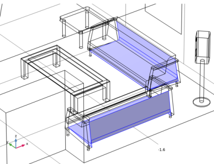
On the object dsp1, select Boundaries 30–33, 156, 189, 195, 196, 265, and 280 only. These are faces on the back and bottom of the couches.
24
In the Model Builder window, click Geometry 1.
25
In the Tools window for Delete Faces, locate the Delete Faces section.
26
Click Delete Selected.
The geometry is now ready for the setting up the simulation. Before defining the physics create selections to make the set-up easier.
Adjacent Selection 1 (adjsel1)
1
In the Geometry toolbar, click  Selections and choose Adjacent Selection.
2
In the Settings window for Adjacent Selection, locate the Input Entities section.
3
From the Geometric entity level list, choose Boundary.
4
5
In the Add dialog box, select Floors:Generic-12" in the Input selections list.
6
7
In the Settings window for Adjacent Selection, locate the Resulting Selection section.
8
From the Show in physics list, choose Off.
Couches
1
In the Geometry toolbar, click  Selections and choose Difference Selection.
2
In the Settings window for Difference Selection, type Couches in the Label text field.
3
Locate the Geometric Entity Level section. From the Level list, choose Boundary.
4
Locate the Input Entities section. Click  Add.
5
In the Add dialog box, select Furniture:M_Sofa-Pensi:2134mm in the Selections to add list.
6
7
In the Settings window for Difference Selection, locate the Input Entities section.
8
9
In the Add dialog box, select Adjacent Selection 1 in the Selections to subtract list.
10
The Couches selection contains only the soft parts of the couches, the legs are excluded.
Woofer Units
1
In the Geometry toolbar, click  Selections and choose Explicit Selection.
2
In the Settings window for Explicit Selection, type Woofer Units in the Label text field.
3
Locate the Entities to Select section. From the Geometric entity level list, choose Boundary.
4
On the object dfa1, select Boundaries 237 and 239 only. These are the boundaries that represent the woofer units of the loudspeakers.
Roof and Walls
1
In the Geometry toolbar, click  Selections and choose Union Selection.
2
In the Settings window for Union Selection, type Roof and Walls in the Label text field.
3
Locate the Geometric Entity Level section. From the Level list, choose Boundary.
4
Locate the Input Entities section. Click  Add.
5
In the Add dialog box, in the Selections to add list, choose Roofs:Generic-12", Walls:BasicWall:Generic-8", and Walls:BasicWall:Interior-5"Partition(2-hr).
6
Doors and Windows
1
In the Geometry toolbar, click  Selections and choose Union Selection.
2
In the Settings window for Union Selection, type Doors and Windows in the Label text field.
3
Locate the Geometric Entity Level section. From the Level list, choose Boundary.
4
Locate the Input Entities section. Click  Add.
5
In the Add dialog box, in the Selections to add list, choose Surface:Doors:M_Double-Glass2:1830x2134mm, Surface:Walls:CurtainWall:CurtainWall1, Surface:Windows:M_CasementDblwithTrim:1220x1220mm, and Surface:Windows:M_Skylight:0610x0686mm.
6
Tables and Stands
1
In the Geometry toolbar, click  Selections and choose Union Selection.
2
In the Settings window for Union Selection, type Tables and Stands in the Label text field.
3
Locate the Geometric Entity Level section. From the Level list, choose Boundary.
4
Locate the Input Entities section. Click  Add.
5
In the Add dialog box, in the Selections to add list, choose Furniture:M_Entertainmentcenter:1830x1830x0610mm, Furniture:M_Table-Coffee:0915x1830x0457mm, Furniture:M_Table-End:0762x0762mm, and Furniture:M_TVStand:M_TVStand.
6
7
In the Geometry toolbar, click  Build All.
Global Definitions
Continue with loading the parameters used for the physics and mesh definitions.
Parameters 1
1
In the Model Builder window, under Global Definitions click Parameters 1.
2
In the Settings window for Parameters, locate the Parameters section.
3
Click  Load from File.
4
Add Material
Add air as the material for the room volume.
1
In the Home toolbar, click  Add Material to open the Add Material window.
2
Go to the Add Material window.
3
4
Click Add to Component in the window toolbar.
5
In the Home toolbar, click  Add Material to close the Add Material window.
Pressure Acoustics, Frequency Domain (acpr)
Normal Acceleration 1
1
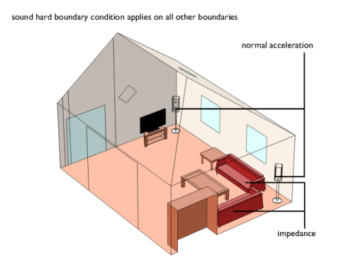
In the Model Builder window, under Component 1 (comp1) right-click Pressure Acoustics, Frequency Domain (acpr) and choose Normal Acceleration.
2
In the Settings window for Normal Acceleration, locate the Boundary Selection section.
3
From the Selection list, choose Woofer Units.
4
Locate the Normal Acceleration section. In the an text field, type Nacc.
Impedance 1
1
In the Physics toolbar, click  Boundaries and choose Impedance.
2
In the Settings window for Impedance, locate the Boundary Selection section.
3
From the Selection list, choose Couches.
4
Locate the Impedance section. In the Zi text field, type Zicouch.
Mesh 1
For acoustics simulations it is important that the mesh resolves the acoustic wavelength, which translates into at least 5 second order elements per wavelength. Specify the maximum allowed mesh size in the domain to comply with this requirement.
1
In the Model Builder window, under Component 1 (comp1) click Mesh 1.
2
In the Settings window for Mesh, locate the Mesh Settings section.
3
From the Sequence type list, choose User-controlled mesh.
Size
1
In the Model Builder window, under Component 1 (comp1)>Mesh 1 click Size.
2
In the Settings window for Size, locate the Element Size section.
3
Click the Custom button.
4
Locate the Element Size Parameters section. In the Maximum element size text field, type lambda0/6.
5
In the Minimum element size text field, type 100[mm].
6
In the Resolution of narrow regions text field, type 0.8.
Size 1
1
In the Model Builder window, right-click Free Tetrahedral 1 and choose Size.
2
In the Settings window for Size, locate the Geometric Entity Selection section.
3
From the Geometric entity level list, choose Boundary.
4
From the Selection list, choose Furniture.
5
Locate the Element Size section. Click the Custom button.
6
Locate the Element Size Parameters section. Select the Maximum element size check box.
7
8
Select the Minimum element size check box.
9
10
Click  Build All.
To view the mesh on the interior boundaries hide some of the wall boundaries.
11
Click the  Click and Hide button in the Graphics toolbar.
12
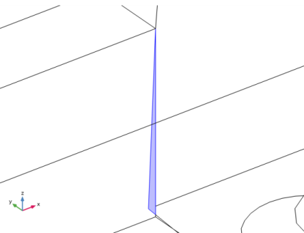
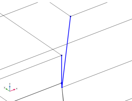
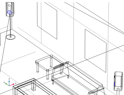
In the Graphics window, click on boundaries 1, 2, 4, 5, 6, 15, 43, and 117 to get a view similar to the figure below.
13
Click the  Click and Hide button in the Graphics toolbar.
Study 1 Frequency Domain
1
In the Model Builder window, click Study 1.
2
In the Settings window for Study, type Study 1 Frequency Domain in the Label text field.
Step 1: Frequency Domain
1
In the Model Builder window, under Study 1 Frequency Domain click Step 1: Frequency Domain.
2
In the Settings window for Frequency Domain, locate the Study Settings section.
3
In the Frequencies text field, type f0.
For large acoustic models it is efficient to use an iterative solver. Switch from the default solver to a recommended iterative solver.
Solution 1 (sol1)
1
In the Study toolbar, click  Show Default Solver.
2
In the Model Builder window, expand the Solution 1 (sol1) node.
3
In the Model Builder window, expand the Study 1 Frequency Domain>Solver Configurations>Solution 1 (sol1)>Stationary Solver 1 node.
4
Right-click Suggested Iterative Solver (GMRES with GMG) (acpr) and choose Enable.
5
In the Study toolbar, click  Compute.
Results
Plots of the acoustic pressure and the sound pressure level are generated by default. Add a multislice plot for a better visualization of the sound pressure level in the room.
Sound Pressure Level (acpr)
1
In the Model Builder window, under Results click Sound Pressure Level (acpr).
2
In the Settings window for 3D Plot Group, locate the Color Legend section.
3
Select the Show maximum and minimum values check box.
Surface 1
1
In the Model Builder window, expand the Sound Pressure Level (acpr) node.
2
Right-click Surface 1 and choose Delete.
Sound Pressure Level (acpr)
In the Model Builder window, click Sound Pressure Level (acpr).
Multislice 1
1
In the Sound Pressure Level (acpr) toolbar, click  More Plots and choose Multislice.
2
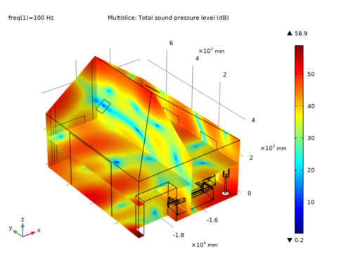
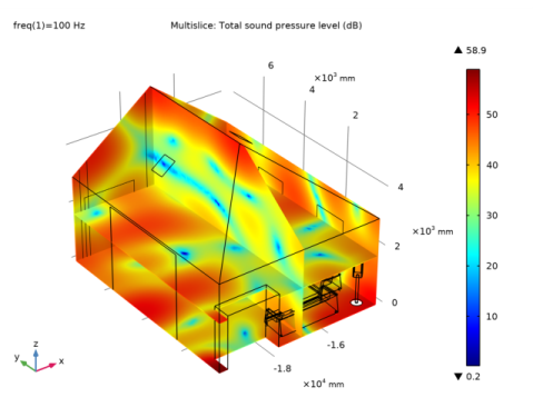
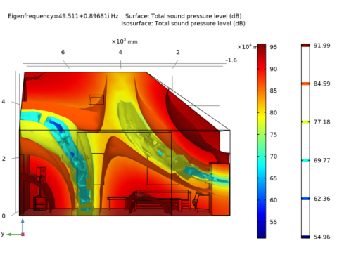
In the Settings window for Multislice, click Replace Expression in the upper-right corner of the Expression section. From the menu, choose Component 1 (comp1)>Pressure Acoustics, Frequency Domain>Pressure and sound pressure level>acpr.Lp_t - Total sound pressure level - dB.
3
Locate the Multiplane Data section. Find the X-planes subsection. From the Entry method list, choose Coordinates.
4
In the Coordinates text field, type -14181 -17000.
5
Find the Y-planes subsection. From the Entry method list, choose Coordinates.
6
In the Coordinates text field, type 7542.
7
Find the Z-planes subsection. From the Entry method list, choose Coordinates.
8
In the Coordinates text field, type 0 1700.
9
In the Sound Pressure Level (acpr) toolbar, click  Plot.
Intensity
Now add a streamline plot of the sound intensity to visualize the flow of energy from the sound sources.
1
In the Home toolbar, click  Add Plot Group and choose 3D Plot Group.
2
In the Settings window for 3D Plot Group, type Intensity in the Label text field.
Streamline 1
1
In the Intensity toolbar, click  Streamline.
2
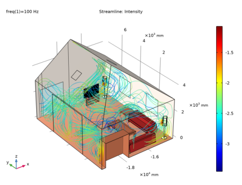
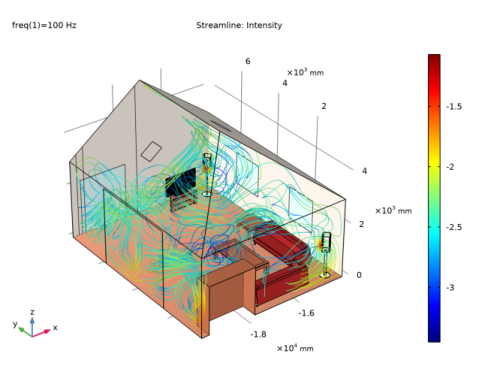
In the Settings window for Streamline, click Replace Expression in the upper-right corner of the Expression section. From the menu, choose Component 1 (comp1)>Pressure Acoustics, Frequency Domain>Intensity>acpr.Ix,acpr.Iy,acpr.Iz - Intensity.
3
Locate the Streamline Positioning section. In the Number text field, type 80.
4
Locate the Selection section. From the Selection list, choose Woofer Units.
5
Locate the Coloring and Style section. Find the Line style subsection. From the Type list, choose Tube.
6
In the Tube radius expression text field, type 10.
7
Select the Radius scale factor check box.
Color Expression 1
1
In the Intensity toolbar, click  Color Expression.
2
In the Settings window for Color Expression, locate the Expression section.
3
In the Expression text field, type log10(acpr.p_t).
4
In the Intensity toolbar, click  Plot.
Intensity
In the Model Builder window, click Intensity.
Surface 1
1
In the Intensity toolbar, click  Surface.
2
In the Settings window for Surface, locate the Expression section.
3
In the Expression text field, type 1.
4
Click to expand the Title section. From the Title type list, choose None.
5
Locate the Coloring and Style section. From the Coloring list, choose Uniform.
6
From the Color list, choose Custom.
7
8
Click Define custom colors.
9
10
Click Add to custom colors.
11
Click Show color palette only or OK on the cross-platform desktop.
Selection 1
1
In the Intensity toolbar, click  Selection.
2
In the Settings window for Selection, locate the Selection section.
3
From the Selection list, choose Roof and Walls.
Surface 2
1
In the Model Builder window, under Results>Intensity right-click Surface 1 and choose Duplicate.
2
In the Settings window for Surface, locate the Coloring and Style section.
3
4
Click Define custom colors.
5
6
Click Add to custom colors.
7
Click Show color palette only or OK on the cross-platform desktop.
Selection 1
1
In the Model Builder window, expand the Surface 2 node, then click Selection 1.
2
In the Settings window for Selection, locate the Selection section.
3
From the Selection list, choose Doors and Windows.
Surface 3
1
In the Model Builder window, under Results>Intensity right-click Surface 2 and choose Duplicate.
2
In the Settings window for Surface, locate the Coloring and Style section.
3
4
Click Define custom colors.
5
6
Click Add to custom colors.
7
Click Show color palette only or OK on the cross-platform desktop.
Selection 1
1
In the Model Builder window, expand the Surface 3 node, then click Selection 1.
2
In the Settings window for Selection, locate the Selection section.
3
From the Selection list, choose Floors:Generic-12".
Surface 4
1
In the Model Builder window, under Results>Intensity right-click Surface 3 and choose Duplicate.
2
In the Settings window for Surface, locate the Coloring and Style section.
3
4
Click Define custom colors.
5
6
Click Add to custom colors.
7
Click Show color palette only or OK on the cross-platform desktop.
Selection 1
1
In the Model Builder window, expand the Surface 4 node, then click Selection 1.
2
In the Settings window for Selection, locate the Selection section.
3
From the Selection list, choose Tables and Stands.
Surface 5
1
In the Model Builder window, under Results>Intensity right-click Surface 4 and choose Duplicate.
2
In the Settings window for Surface, locate the Coloring and Style section.
3
4
Click Define custom colors.
5
6
Click Add to custom colors.
7
Click Show color palette only or OK on the cross-platform desktop.
Selection 1
1
In the Model Builder window, expand the Surface 5 node, then click Selection 1.
2
In the Settings window for Selection, locate the Selection section.
3
From the Selection list, choose Couches.
Surface 6
1
In the Model Builder window, under Results>Intensity right-click Surface 5 and choose Duplicate.
2
In the Settings window for Surface, locate the Coloring and Style section.
3
From the Color list, choose Black.
Selection 1
1
In the Model Builder window, expand the Surface 6 node, then click Selection 1.
2
In the Settings window for Selection, locate the Selection section.
3
From the Selection list, choose Furniture:M_TV-FlatScreen:1270mm.
Intensity
Add Study
1
In the Home toolbar, click  Add Study to open the Add Study window.
2
Go to the Add Study window.
3
Find the Studies subsection. In the Select Study tree, select General Studies>Eigenfrequency.
4
Click Add Study in the window toolbar.
5
In the Home toolbar, click  Add Study to close the Add Study window.
Study 2
Step 1: Eigenfrequency
1
In the Settings window for Eigenfrequency, locate the Study Settings section.
2
In the Search for eigenfrequencies around text field, type 10[Hz].
3
From the Eigenfrequency search method around shift list, choose Larger real part.
4
In the Model Builder window, click Study 2.
5
In the Settings window for Study, type Study 2 Eigenfrequency in the Label text field.
Solution 2 (sol2)
1
In the Study toolbar, click  Show Default Solver.
2
In the Model Builder window, expand the Solution 2 (sol2) node.
3
In the Model Builder window, expand the Study 2 Eigenfrequency>Solver Configurations>Solution 2 (sol2)>Eigenvalue Solver 1 node.
4
Right-click Suggested Iterative Solver (GMRES with GMG) (acpr) and choose Enable.
5
In the Study toolbar, click  Compute.
Results
Sound Pressure Level (acpr) 1
1
In the Model Builder window, under Results click Sound Pressure Level (acpr) 1.
2
In the Settings window for 3D Plot Group, locate the Data section.
3
From the Eigenfrequency (Hz) list, choose 49.511+0.89681i.
Isosurface 1
1
In the Sound Pressure Level (acpr) 1 toolbar, click  Isosurface.
2
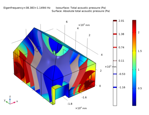
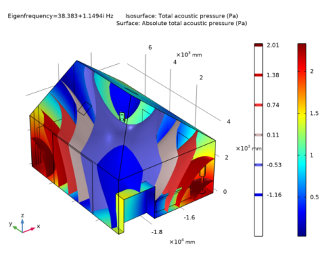
In the Settings window for Isosurface, click Replace Expression in the upper-right corner of the Expression section. From the menu, choose Component 1 (comp1)>Pressure Acoustics, Frequency Domain>Pressure and sound pressure level>acpr.Lp_t - Total sound pressure level - dB.
3
Locate the Levels section. In the Total levels text field, type 6.
4
In the Sound Pressure Level (acpr) 1 toolbar, click  Plot.
5
Click the  Go to YZ View button in the Graphics toolbar.
6
Click the  Go to YZ View button in the Graphics toolbar.
7
Click the  Go to YZ View button in the Graphics toolbar.
Acoustic Pressure, Isosurfaces (acpr) 1
1
In the Model Builder window, click Acoustic Pressure, Isosurfaces (acpr) 1.
2
In the Settings window for 3D Plot Group, locate the Data section.
3
From the Eigenfrequency (Hz) list, choose 38.383+1.1494i.
Isosurface 1
1
In the Model Builder window, expand the Acoustic Pressure, Isosurfaces (acpr) 1 node, then click Isosurface 1.
2
In the Settings window for Isosurface, locate the Levels section.
3
In the Total levels text field, type 6.
Acoustic Pressure, Isosurfaces (acpr) 1
In the Model Builder window, click Acoustic Pressure, Isosurfaces (acpr) 1.
Surface 1
1
In the Acoustic Pressure, Isosurfaces (acpr) 1 toolbar, click  Surface.
2
In the Settings window for Surface, click Replace Expression in the upper-right corner of the Expression section. From the menu, choose Component 1 (comp1)>Pressure Acoustics, Frequency Domain>Pressure and sound pressure level>acpr.absp_t - Absolute total acoustic pressure - Pa.
3
In the Acoustic Pressure, Isosurfaces (acpr) 1 toolbar, click  Plot.
4
Click the  Go to Default View button in the Graphics toolbar.