PDF

Domain Activation and Deactivation
Introduction
Heating of an object from alternating regions is one example where the modeling technique of activating and deactivating physics on domains can be useful. This example demonstrates how you can apply this technique using the LiveLink™ for MATLAB®.
Model Definition
Assume that you want to study the heat distribution in a larger copper plate as it is heated by a steel plate that is moved between various locations. The hot steel plate remains in each spot on the base plate for two minutes before being moved to the next.
In Figure 1 the copper plate is shown in orange. All four locations of the steel plate are present in the geometry, but only one of those is active at any given time. Assume that the hot plate moves instantaneously every two minutes by deactivating the old and activating a new domain in the figure. The active domains are shown in blue, and are also marked with a filled circle.
The heat is conducted between the steel plate, with an initial temperature of 500 K, and the copper plate through a thin thermally resistive layer. The copper plate is cooled by the surrounding air, a process which you model with convective cooling using a heat transfer coefficient.
Figure 1: Model geometry with the copper plate in orange and the active steel plate in blue marked by a filled circle.
Results and Discussion
Figure 2 shows the temperature at two of the corners and in the middle of the top surface of the copper plate. While the temperature is increasing at all three locations the corners show a larger fluctuation in temperature due to the steel plate alternating between locations close by or further away from the points.
Figure 2: The temperature at two of the corners and in the middle of the top surface of the copper plate.
You can follow the temperature distribution in the copper plate as it heats up during the time frame of the simulation in Figure 3.
Figure 3: Temperature distribution in the copper plate.
Notes About the COMSOL Implementation
In addition to the activation and deactivation of domains this example demonstrates other important modeling techniques, namely
The most efficient approach for this simulation is to start by setting up the heat transfer problem in the graphical user interface of the COMSOL Desktop®. You can then save the model *.mph file, which you can easily load into MATLAB®, where you continue to implement the script for solving the model.
Wrapper functions used by the script:
mphopen to load the model .mph file.
mphglobal to evaluate global quantities in the model.
mphplot to display plots.
Application Library path: LiveLink_for_MATLAB/Tutorials/domain_activation_llmatlab
Modeling Instructions — MATLAB®
In this section you find a detailed explanation of the commands you need to enter at the MATLAB command line in order to run the simulation.
1
Start COMSOL with MATLAB.
You now have two possibilities to continue:
Enter each command, starting at step 2 below, at the MATLAB command line.
Paste the full model script, included in the section Model M-File, into a text editor, then save the file with a “.m” extension, and finally run this file in MATLAB.
2
model = mphopen('domain_activation_llmatlab');
Note: See the section Modeling Instructions — COMSOL Desktop for the modeling instruction of the model .mph file domain_activation_llmatlab.mph.
3
domInd = [2,3,5,4];
4
ht = model.physics('ht');
5
for i = 1:8
6
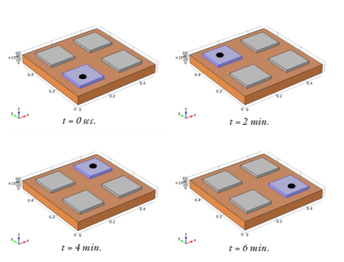
The next command defines the variable k as the modulus of the division of the iteration number by 8. Use this variable in step 8 below to define which domain becomes active in the current iteration.
k = mod(i,4);
7
if k == 0
   k = 4;
end
8
The heat transfer physics interface should be active only on the copper plate, domain 1, and the currently active steel plate, domain k. Set the domain selection for the heat transfer physics interface, and initial condition feature node 'init2' according to the following:
ht.selection.set([1 domInd(k)]);
ht.feature('init2').selection.set(domInd(k));
9
model.study('std1').run;
Once the solution of the first iteration is computed you need make some changes in the model object before continuing the analysis.
10
if i==1
   cpt1 = model.result.dataset.create('cpt1', 'CutPoint3D');
   cpt1.set('pointx', '0 L/2 L');
   cpt1.set('pointy', '0 L/2 L');
   cpt1.set('pointz', 'L/10');
   pg1 = model.result.create('pg1', 'PlotGroup1D');
   pg1.set('data', 'cpt1');
   ptgr1 = pg1.feature.create('ptgr1', 'PointGraph');
   ptgr1.set('legend', 'on');
11
   pg2 = model.result.create('pg2', 'PlotGroup3D');
   surf1 = pg2.feature.create('surf1', 'Surface');
   surf1.set('rangecoloractive', 'on');
   surf1.set('rangecolormax', '336');
   surf1.set('rangecolormin', '293.15');
12
   ht.feature('init1').set('T', 1, 'T');
13
   v1 = model.sol('sol1').feature('v1');
   v1.set('initsol', 'sol1');
end
The following steps apply to all iterations.
14
figure(1)
mphplot(model,'pg1','rangenum',1)
hold on
15
figure(2)
subplot(4,2,i)
pg2.setIndex('looplevel','25',0)
mphplot(model,'pg2');
16
Use the function mphglobal to extract the value of the simulation stop time of the current iteration. Use this to update the solver start time for the next iteration:
time = mphglobal(model,'t','solnum','end');
model.param.set('t0',time);
17
disp(sprintf('End of iteration No.%d',i));
end
Model M-File
Below you find the full script of the model. You can copy it and paste it into a text editor and save it with the “.m” extension. To run the script in MATLAB make sure that the path to the folder containing the script is set in MATLAB, then type the file name without the “.m” extension at the MATLAB prompt.
model = mphopen('domain_activation_llmatlab');
 
domInd = [2,3,5,4];
ht = model.physics('ht');
 
for i = 1:8
   k = mod(i,4);
   if k == 0
      k = 4;
   end
   ht.selection.set([1 domInd(k)]);
   ht.feature('init2').selection.set(domInd(k));
 
   model.study('std1').run;
 
   if i==1
      cpt1 = model.result.dataset.create('cpt1', 'CutPoint3D');
      cpt1.set('pointx', '0 L/2 L');
      cpt1.set('pointy', '0 L/2 L');
      cpt1.set('pointz', 'L/10');
      pg1 = model.result.create('pg1', 'PlotGroup1D');
      pg1.set('data', 'cpt1');
      ptgr1 = pg1.feature.create('ptgr1', 'PointGraph');
      ptgr1.set('legend', 'on');
      pg2 = model.result.create('pg2', 'PlotGroup3D');
      surf1 = pg2.feature.create('surf1', 'Surface');
      surf1.set('rangecoloractive', 'on');
      surf1.set('rangecolormax', '336');
      surf1.set('rangecolormin', '293.15');
            
      ht.feature('init1').set('T', 1, 'T');
 
      v1 = model.sol('sol1').feature('v1');
      v1.set('initsol', 'sol1');
   end
 
   figure(1)
   mphplot(model,'pg1','rangenum',1)
   hold on
 
   figure(2)
   subplot(4,2,i)
   pg2.setIndex('looplevel','25',0);
   mphplot(model,'pg2');
 
   time = mphglobal(model,'t','solnum','end');
   model.param.set('t0',time);
 
   disp(sprintf('End of iteration No.%d',i));
end
Modeling Instructions — COMSOL Desktop
Use the COMSOL Desktop to set-up the heat transfer simulation. You can later load this example into MATLAB, using LiveLink™, to continue the model implementation.
From the File menu, choose New.
New
In the New window, click  Model Wizard.
Model Wizard
1
In the Model Wizard window, click  3D.
2
In the Select Physics tree, select Heat Transfer>Heat Transfer in Solids (ht).
3
Click Add.
4
Click  Study.
5
In the Select Study tree, select General Studies>Time Dependent.
6
Global Definitions
Parameters 1
1
In the Model Builder window, under Global Definitions click Parameters 1.
2
In the Settings window for Parameters, locate the Parameters section.
3
Geometry 1
Block 1 (blk1)
1
In the Geometry toolbar, click  Block.
2
In the Settings window for Block, locate the Size and Shape section.
3
In the Width text field, type L.
4
In the Depth text field, type L.
5
In the Height text field, type L/10.
Block 2 (blk2)
1
In the Geometry toolbar, click  Block.
2
In the Settings window for Block, locate the Size and Shape section.
3
In the Width text field, type l.
4
In the Depth text field, type l.
5
In the Height text field, type l/10.
6
Locate the Position section. In the x text field, type L/10.
7
In the y text field, type L/10.
8
In the z text field, type L/10.
Array 1 (arr1)
1
In the Geometry toolbar, click  Transforms and choose Array.
2
3
In the Settings window for Array, locate the Size section.
4
In the x size text field, type 2.
5
In the y size text field, type 2.
6
Locate the Displacement section. In the x text field, type L/2.
7
In the y text field, type L/2.
Form Union (fin)
In the Model Builder window, right-click Form Union (fin) and choose Build Selected.
Materials
In the Materials toolbar, click  Browse Materials.
Material Browser
1
In the Material Browser window, select Built-in>Structural steel in the tree.
2
Click  Add to Component.
3
In the tree, select Built-in>Copper.
4
Click  Add to Component.
5
6
Definitions
Box 1
1
In the Definitions toolbar, click  Box.
2
In the Settings window for Box, locate the Geometric Entity Level section.
3
From the Level list, choose Boundary.
4
Locate the Box Limits section. In the x minimum text field, type -1e-3.
5
In the x maximum text field, type L+1e-3.
6
In the y minimum text field, type -1e-3.
7
In the y maximum text field, type L+1e-3.
8
In the z minimum text field, type L/10-1e-3.
9
In the z maximum text field, type L/10+1e-3.
10
Locate the Output Entities section. From the Include entity if list, choose Entity inside box.
Heat Transfer in Solids (ht)
Initial Values 2
1
In the Model Builder window, under Component 1 (comp1) right-click Heat Transfer in Solids (ht) and choose Initial Values.
2
3
In the Settings window for Initial Values, locate the Initial Values section.
4
In the T text field, type T0.
Heat Flux 1
1
In the Physics toolbar, click  Boundaries and choose Heat Flux.
2
In the Settings window for Heat Flux, locate the Boundary Selection section.
3
From the Selection list, choose Box 1.
4
Locate the Heat Flux section. Click the Convective heat flux button.
5
In the h text field, type h0.
Thin Layer 1
1
In the Physics toolbar, click  Boundaries and choose Thin Layer.
2
In the Settings window for Thin Layer, locate the Boundary Selection section.
3
From the Selection list, choose Box 1.
4
Locate the Heat Conduction section. From the k list, choose User defined. In the associated text field, type ks.
5
Locate the Thermodynamics section. From the ρ list, choose User defined. From the Cp list, choose User defined.
Materials
Material 3 (mat3)
1
In the Model Builder window, under Component 1 (comp1) right-click Materials and choose Layers>Single Layer Material.
2
In the Settings window for Material, locate the Geometric Entity Selection section.
3
From the Selection list, choose Box 1.
4
Locate the Material Contents section. In the table, enter the following settings:
Mesh 1
Free Quad 1
1
In the Mesh toolbar, click  Boundary and choose Free Quad.
2
In the Settings window for Free Quad, locate the Boundary Selection section.
3
From the Selection list, choose Box 1.
Swept 1
In the Mesh toolbar, click  Swept.
Distribution 1
1
Right-click Swept 1 and choose Distribution.
2
3
In the Settings window for Distribution, locate the Distribution section.
4
In the Number of elements text field, type 2.
Distribution 2
1
In the Model Builder window, right-click Swept 1 and choose Distribution.
2
3
In the Settings window for Distribution, locate the Distribution section.
4
In the Number of elements text field, type 3.
Size
1
In the Model Builder window, click Size.
2
In the Settings window for Size, locate the Element Size section.
3
From the Predefined list, choose Finer.
4
Click  Build All.
Study 1
Step 1: Time Dependent
1
In the Model Builder window, under Study 1 click Step 1: Time Dependent.
2
In the Settings window for Time Dependent, locate the Study Settings section.
3
In the Output times text field, type range(t0,dt,tf).
Save the Model
1
2
Browse to a directory which path is set in MATLAB and enter domain_activation_llmatlab in the File name text field.
3
Click Save.