Geometric Parameter Optimization of a Tuning Fork

Tuning forks have traditionally been used for tuning of musical instruments due to their ability to sound a very pure tone at their fundamental eigenfrequency. To design a tuning fork that sounds the note A, 440 Hz, you first compute the fundamental eigenfrequency and eigenmode for a design with a prong length estimated from theory. Then you use geometric parameter optimization to fine tune the prong size so that the fundamental eigenfrequency corresponds to 440 Hz.

Model Definition

The model geometry is shown in Figure 1. The fundamental frequency of the fork is determined by the length of the prongs, the cross-sectional geometry of the prongs, and the material properties of the fork.

Figure 1: Tuning fork geometry.

The following formula gives a theoretical estimation for the fundamental frequency of a tuning fork with cylindrical cross section of the prong (Ref. 1):

(1)

where R2 is the radius of the cross section of the prongs, E denotes Young’s modulus, and ρ is the density. The length of the prong can be estimated as

(2)

where R1 the radius of the base, and L is the length of the straight cylindrical part, see Figure 1.

In the fundamental eigenmode, the prongs move apart and together while the handle moves up and down as shown in Figure 2. Thus, the eigenmode is symmetric with a symmetry plane placed between the prongs.

Figure 2: Vibration of the tuning fork in its fundamental eigenmode.

The advantage with the shape of the fundamental eigenmode is that the relative displacements in the handle are very small, which makes it possible to hold the fork without damping the vibration. This also allows to make use of the theoretical estimation for the frequency Equation 1 which is based on the solution for a cantilever beam representing each prong.

The parameters used in the model are: R1 = 7.5 mm and R2 = 2.5 mm. The fork material is Steel AISI 4340, for which E = 205 GPa and ρ = 7850 kg/m3.

For the frequency f = 440 Hz, Equation 1 and Equation 2 give the length of the prong cylindrical part as L = 7.8 cm. This presents an underestimation because the part of the prong near the base has larger bending stiffness compared to that for a straight cantilever beam.

Results and Discussion

For the prong length of L = 78 mm the simulation results in an eigenfrequency of 457 Hz. This number is higher than expected, since Equation 1 and Equation 2 underestimate the prong length due to the higher stiffness at the base compared to a straight cantilever beam.

Figure 3 shows the mode shape plot for the prong length optimized for the fundamental eigenfrequency of 440 Hz. The optimized length is 79.65 mm, which, as expected, is longer than the from theory estimated 78 mm.

Figure 3: Frequency and mode shape of the fundamental eigenmode for the optimized tuning fork.

Notes About the COMSOL Implementation

The tuning fork geometry you are using in this model comes from an Inventor design. Using LiveLink for Inventor you synchronize the geometry and the parameter for the tuning fork prong length between Inventor and COMSOL Multiphysics. In order for this to work you need to have both programs running during modeling, and you need to make sure that the tuning fork file is the active file in Inventor.

Reference

1. Tuning fork, http://en.wikipedia.org/wiki/Tuning_fork

LiveLink_for_Inventor/Tutorials,_LiveLink_Interface/tuning_fork_llinventor

Modeling Instructions

You can set up this simulation both by working inside Inventor, using the embedded COMSOL simulation environment, and by working in the standalone COMSOL Desktop. Regardless which way you proceed, first you need to open the CAD file with the geometry in Inventor.

In Inventor open the file tuning_fork.ipt located in the model’s Application Library folder.

Switch to the COMSOL Desktop, and skip the next section. Or, continue below if you are working inside Inventor.

Modeling Inside Inventor

On the tab click the button.

In case it is not already running, the COMSOL modeling environment will be started, and the geometry will be synchronized automatically.

Continue with step 2 under the Model Wizard section.

COMSOL Desktop

From the menu, choose .

New

In the window, click

Model Wizard

In the window, click

In the tree, select .

Click .

Click

In the tree, select .

Click

Geometry 1

The geometry is already synchronized if you are modeling inside Inventor, and you can skip to step 4 in the section LiveLink for Inventor 1 (cad1).

Make sure that the CAD Import Module kernel is used.

In the window, under click .

In the window for , locate the section.

From the list, choose .

LiveLink for Inventor 1 (cad1)

Right-click and choose .

In the window for , locate the section.

Click .

After a few moments the geometry of the tuning fork appears in the window.

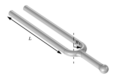
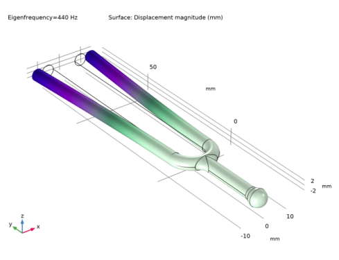
Click to expand the section. The dimensional parameter for the prong length, d1 in the Inventor file, has been linked to COMSOL Multiphysics and is therefore synchronized with the geometry. To manage linked parameters, you can click on the tab in Inventor. The global parameter, LL_d1, is automatically generated in the COMSOL Multiphysics model during synchronization to enable parametric sweeps and optimization of the geometry.

Global Definitions

Parameters 1

In the window, under click .

In the window for , locate the section.

In the table, enter the following settings:


Name	Expression	Value	Description
LL_d1	78[mm]	0.078 m

Geometry 1

LiveLink for Inventor 1 (cad1)

In the window, under click .

In the window for , locate the section.

Click ( if you are setting up the model inside Inventor).

Materials

Add Material

From the menu, choose .

Add Material

Go to the window.

In the tree, select .

Click the right end of the split button in the window toolbar.

From the menu, choose .

Mesh 1

Size

In the window, under right-click and choose .

Free Tetrahedral 1

Change the default mesh settings to get a finer mesh that better resolves the geometry.

Size 1

In the window, right-click and choose .

In the window for , locate the section.

From the list, choose .

Locate the section. From the list, choose .

Study 1

Step 1: Eigenfrequency

Set up the study to search for the fundamental eigenfrequency.

In the window, under click .

In the window for , locate the section.

Select the check box.

In the associated text field, type 1.

In the text field, type 440[Hz].

In the window, right-click and choose .

Results

Mode Shape (solid)

After the computation is finished a plot similar to the one below appears.

Study 1

Continue with setting up the optimization.

Optimization

Right-click and choose .

In the window for , locate the section.

From the list, choose .

Locate the section. In the table, enter the following settings:


Expression	Description	Evaluate for
abs(freq-440)	Frequency	Eigenfrequency

Locate the section. Click

In the table, enter the following settings:


Parameter name	Initial value	Scale	Lower bound	Upper bound
LL_d1	78[mm]	0.01	78[mm]	81[mm]

Right-click and choose .

Results

Mode Shape (solid)

After the optimization is finished a plot similar to Figure 3 is displayed. You can read the value of the eigenfrequency from the plot. Continue with displaying the value of the optimized prong length parameter in a table.

Global Evaluation 1

In the window, right-click and choose .

In the window for , click in the upper-right corner of the section. From the menu, choose .

Click

Geometry 1

LiveLink for Inventor 1 (cad1)

In the window, under click .

In the window for , locate the section.

Click in the upper-right corner of the section.

Form Union (fin)

In the window, click .

In the window for , click