Geometric Parameter Optimization of a Bracket

In some application fields, there is a strong focus on weight reduction. For example, this is the case in the automotive industry, where every gram has a distinct price tag.

The bracket is used for mounting a heavy component on a vibrating foundation. It is thus important to keep the natural frequency well above the excitation frequency in order to avoid resonances. The bracket is also subjected to shock loads, which can be treated as a static acceleration load. This gives an optimization problem, where results from two different study types must be considered simultaneously.

By using the LiveLink interface for Inventor the weight of a mounting bracket is reduced, given an upper bound on the stresses and a lower bound on the first natural frequency. The model demonstrates how to synchronize the geometry between Inventor and COMSOL Multiphysics while updating dimensional parameters, and how to perform an optimization study.

This application requires the Optimization Module, the Structural Mechanics Module, and the LiveLink interface for Inventor.

Model Definition

The original bracket together with a sketched mounted component are shown in Figure 1. The bracket is made of steel.

The component, which can be considered as rigid when compared with the bracket, has its center of gravity at the center of the circular cutout in the bracket. The mass is 4.4 kg, the moment of inertia around its longitudinal axis is 7.1·10−4 kg·m2, and the moment of inertia around the two transverse axes is 9.3·10−4 kg·m2.

Figure 1: Bracket supporting a heavy component.

The idea is to reduce the weight by drilling holes in the vertical surface of the bracket, and at the same time change the dimensions of the indentations, in order to offset the loss in stiffness.

Optimization Parameters

Six geometrical parameters are used in the optimization. They are summarized in Table 1 and shown in Figure 2.

Table 1: Geometrical parameters.
Parameter	Description	Lower limit (mm)	Upper limit (mm)
RC	Radius of the central hole	3	15
ZCO	Vertical distance from the bend to the edge of the central hole	1	23
RO	Radius of the outer hole	3	15
ZOO	Vertical distance from the bend to the edge of the outer hole	8	30
YOO	Horizontal distance from the edge of the bracket to outer hole	3	29
WIND	Width of the indentation	8	20

Figure 2: Optimization parameters.

Constraints

•

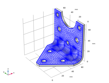
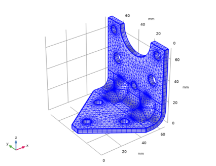
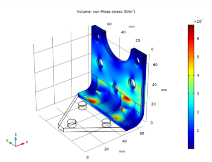
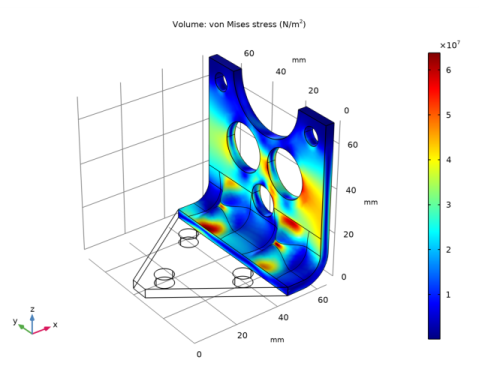
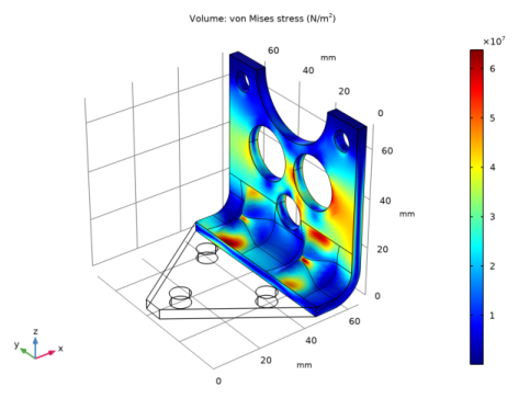
The lowest natural frequency must be at least 60 Hz.

•

When exposed to a peak acceleration of 4g in all three global directions simultaneously, the effective stress is not allowed to exceed 80 MPa anywhere. This criterion is nondifferentiable, because the location of the peak stress can jump from one place to another. A gradient-free optimization algorithm must thus be used.

•

There must be at least 3 mm of material between two holes, or between a hole and an edge. This criterion is enforced both through the limits on the control parameters and as constraints. The geometrical constraints are shown in Figure 3.

Figure 3: Geometrical constraints.

The COBYLA solver uses sampling in the control variable space to approximate both the objective function, the constraints, and the control variable bounds. Individual samples may be computed outside the bounds and in violation of the constraints. Therefore, it is important to parameterize the geometry in such a way that it is robust with respect to (small) constraint and bound violations.

Bounds and linear constraints are generally satisfied to high precision at the optimum point returned by the solver, but nonlinear constrains are often slightly violated. The reason is that the solver tends to converge from the outside of the feasible domain and terminates before the constraints are completely satisfied. Tightening the solver tolerances will decrease the constraint violation but is often not worth the computational effort; it is better to specify constraints with a safety margin.

Results and Discussion

The initial geometry used in the optimization is shown in Figure 4. Three rather small holes have been introduced.

Figure 4: Initial geometry.

The optimal values of the geometrical parameters are shown in Table 2.

Table 2: Optimal values.
Parameter	Optimal value (mm)	Lower limit (mm)	Upper limit (mm)
LL_RC	7.34	3	15
LL_ZCO	1	1	23
LL_RO	10.76	3	15
LL_YOO	11.25	3	29
LL_ZOO	16.37	8	30

The weight of the optimized bracket is about 179 g, a reduction of 21 g from the original 200.57 g. The stresses from the shock load on the optimized geometry are shown in Figure 5

Figure 5: Stresses at peak load in the optimized design.

The optimal solution gives three fairly large holes, and the widest possible indentation.

There are several possible arrangements of the holes that give the same weight reduction within a small tolerance. It is therefore possible that the design variables are not always the same at convergence.

Notes About the COMSOL Implementation

The bracket geometry you are using in this model comes from an Inventor design. Using LiveLink for Inventor you synchronize the geometry and parameters for the dimension of the bracket and the positioning of holes between Inventor and COMSOL Multiphysics. In order for this to work you need to have both programs running during modeling, and you need to make sure that the bracket file is the active file in Inventor.

The component mounted on the bracket is not modeled in detail. It is replaced by a Rigid Connector having the equivalent inertial properties.

LiveLink_for_Inventor/Tutorials,_LiveLink_Interface/bracket_optimization_llinventor

Modeling Instructions

You can set up this simulation both by working inside Inventor, using the embedded COMSOL simulation environment, and by working in the standalone COMSOL Desktop. Regardless which way you proceed, first you need to open the CAD file with the geometry in Inventor.

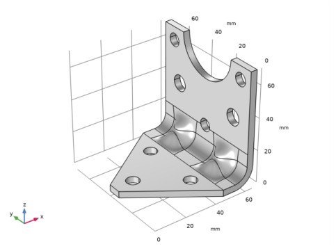
In Inventor open the file bracket_optimization.ipt located in the model’s Application Library folder.

Switch to the COMSOL Desktop, and skip the next section. Or, continue below if you are working inside Inventor.

Modeling Inside Inventor

On the tab click the button.

In case it is not already running, the COMSOL modeling environment will be started, and the geometry will be synchronized automatically.

Continue with step 2 under the Model Wizard section.

COMSOL Desktop

From the menu, choose .

New

In the window, click

Model Wizard

In the window, click

In the tree, select .

Click .

Click

In the tree, select .

Click

Geometry 1

The geometry is already synchronized if you are modeling inside Inventor, and you can skip to step 4 in the section LiveLink for Inventor 1 (cad1).

Make sure that the CAD Import Module kernel is used.

In the window, under click .

In the window for , locate the section.

From the list, choose .

LiveLink for Inventor 1 (cad1)

Right-click and choose .

In the window for , locate the section.

Click .

After a few moments the geometry of the bracket appears in the window.

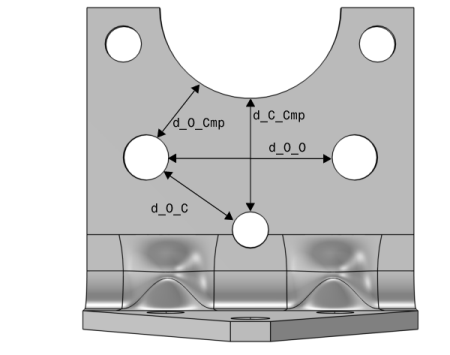
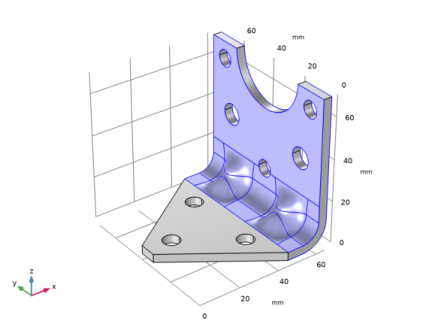
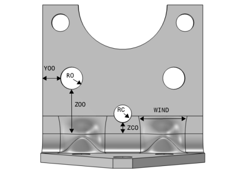
Click to expand the section. The table contains ten dimensions, THK, LX, LZ, DCMP, BDIA, RC, ZCO, RO, YOO and ZOO, which are part of the Inventor model. In Inventor, the button on the tab allows you to select and view dimensions for synchronization. These dimensions are retrieved, and appear in the column of the table. The corresponding entries in the column, LL_THK, LL_LX and so on, are global parameters in the COMSOL model. These are automatically generated during synchronization, and are assigned the values of the linked Inventor dimensions. The parameter values are displayed in the column.

Global parameters in a model allow you to parameterize settings and can be controlled by the optimization solver to perform parametric sweeps. Thus, by linking Inventor dimensions to COMSOL global parameters, the optimization solver can automatically update and synchronize the geometry for each new value in a sweep.

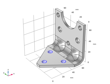
Click to expand the section. The selections listed here are user defined selections saved in the Inventor files for the components that they appear on. In Inventor, you can set-up selections using the button on the tab.

Right-click and choose .

Global Definitions

Parameters 1

In the window, under click .

The table already contains the automatically generated global parameters that are linked to the Inventor dimensions.

Based on the parameters in the table you can define expressions to constrain the positioning of the holes while optimizing the bracket. Later on you will set up the optimization solver to take into account these geometric constraints. Now, continue with loading the expressions for the geometric constraints and the parameters needed to define the physics. Since the parameter file contains all parameters, including the already synchronized ones, clear the table first to avoid duplicates.

In the window for , locate the section.

Click

Browse to the model’s Application Libraries folder and double-click the file bracket_optimization_parameters.txt.

Materials

Add Material

From the menu, choose .

Add Material

Go to the window.

In the tree, select .

Click the right end of the split button in the window toolbar.

From the menu, choose .

Solid Mechanics (solid)

Fixed (Bolts)

In the window, under right-click and choose .

The exact way the bolts clamp the bracket to the foundation is not important for the results in the part being optimized.

In the window for , type Fixed (Bolts) in the text field.

Locate the section. From the list, choose .

Rigid Connector (Mounted component)

In the window, right-click and choose .

The attached component has a high stiffness, and is bolted to the two upper bolt holes. It is modeled as being rigid, with only mass properties.

In the window for , type Rigid Connector (Mounted component) in the text field.

Locate the section. From the list, choose .

Locate the section. From the list, choose .

Specify the Xc vector as


LL_LX-LL_THK/2	x
(4*LL_BDIA+LL_DCMP)/2	y
LL_LZ	z

Mass and Moment of Inertia 1

Right-click and choose .

In the window for , locate the section.

In the m text field, type mCmp.

From the list, choose .

In the I table, enter the following settings:


IXCmp	0	0
0	IYZCmp	0
0	0	IYZCmp

Mesh 1

In the window, under click .

In the window for , locate the section.

From the list, choose .

Free Triangular 1

Right-click and choose .

In the window for , locate the section.

From the list, choose .

Size 1

Right-click and choose .

In the window for , locate the section.

Click the button.

Locate the section. Select the check box.

In the associated text field, type 0.2.

Select the check box.

In the associated text field, type 0.38.

Click

Swept 1

In the window, right-click and choose .

Distribution 1

In the window, right-click and choose .

In the window for , locate the section.

In the text field, type 3.

Click

Eigenfrequency Study

Run an eigenfrequency study on the initial geometry.

In the window, click .

In the window for , type Eigenfrequency Study in the text field.

Click

Solid Mechanics (solid)

Add the peak loads, and perform a stationary study.

Body load 4g on bracket

In the window, under right-click and choose .

In the window for , type Body load 4g on bracket in the text field.

Locate the section. From the list, choose .

Locate the section. Specify the FV vector as


4g_constsolid.rho	x
4g_constsolid.rho	y
4g_constsolid.rho	z

Force 4g on mounted component

In the window, right-click and choose .

In the window for , type Force 4g on mounted component in the text field.

Locate the section. Specify the F vector as


4g_constmCmp	x
4g_constmCmp	y
4g_constmCmp	z

Root

From the menu, choose .

Add Study

Go to the window.

Find the subsection. In the tree, select .

Click in the window toolbar.

From the menu, choose .

Stationary Study

In the window, click .

In the window for , type Stationary Study in the text field.

Click

Definitions

Prepare for the optimization by adding variables for the bracket mass and the maximum stress.

Integration 1 (intop1)

In the window, under right-click and choose .

In the window for , locate the section.

From the list, choose .

Maximum 1 (maxop1)

In the window, right-click and choose .

The boundaries for which the maximum stress is going to be evaluated are defined as in Inventor.

In the window for , locate the section.

From the list, choose .

Variables 1

Right-click and choose .

In the window for , locate the section.

In the table, enter the following settings:


Name	Expression	Unit	Description
mass	intop1(solid.rho)	kg	Bracket mass
maxStress	maxop1(solid.mises)	N/m²	Maximum stress

Results

Add a plot for monitoring the geometry and stresses in the optimized region.

Stress in Optimized Region

In the window, right-click and choose .

In the window for , type Stress in Optimized Region in the text field.

Locate the section. From the list, choose .

Volume 1

Right-click and choose .

In the window for , locate the section.

In the text field, type solid.mises.

Filter 1

Right-click and choose .

In the window for , locate the section.

In the text field, type x>LL_LX-5*LL_THK.

Click the

button in the toolbar.

Set up the optimization study.

Root

From the menu, choose .

Add Study

Go to the window.

Find the subsection. In the tree, select .

Click in the window toolbar.

From the menu, choose .

Optimization Study

In the window for , type Optimization Study in the text field.

Optimization

Right-click and choose .

Eigenfrequency

Right-click and choose .

In the window for , type Eigenfrequency in the text field.

Locate the section. From the list, choose .

Stationary

Right-click and choose .

In the window for , type Stationary in the text field.

Locate the section. From the list, choose .

Optimization

In the window, click .

In the window for , locate the section.

From the list, choose .

Find the subsection. Clear the check box.

Locate the section. Select the check box.

Locate the section. In the table, enter the following settings:


Expression	Description	Evaluate for
comp1.mass	Bracket mass	Stationary

Locate the section. In the text field, type 0.1.

The first eigenfrequency is to be used in the optimization.

Locate the section. From the list, choose .

Locate the section. Click

Browse to the model’s Application Libraries folder and double-click the file bracket_optimization_ctrlvars.txt.

Locate the section. In the table, enter the following settings:


Expression	Lower bound	Upper bound	Evaluate for
real(comp1.solid.freq)	minFreq		Eigenfrequency
comp1.maxStress/maxStressLimit		1	Stationary
d_O_Cmp	3[mm]		Eigenfrequency
d_C_Cmp	3[mm]		Eigenfrequency
d_O_C	3[mm]		Eigenfrequency
d_O_O	3[mm]		Eigenfrequency

Locate the section. Select the check box.

From the list, choose .

If some configurations are not valid, the optimization procedure should still continue. The default is to stop if an error occurs.

Solution 3 (sol3)

In the window, right-click and choose .

Run the optimization.

Right-click and choose .

Results

On the last line of you will find the optimal set of parameters, and the minimum weight. Note that the value in the column can be colored orange if the solution violates a constraint slightly, but is still accepted within the tolerances.

On the last line of you will find the values of the natural frequency and maximum stress in the optimized configuration, as well as the values of the other constraints.

To avoid scrolling through a large number of table entries, insert a which shows only the optimized parameters.

In the table, enter the following settings:


Name	Description
LL_THK	Plate thickness
LL_LX	Bracket length
LL_LZ	Bracket height
LL_DCMP	Diameter of component
LL_BDIA	Diameter of mounting bolts
LL_RC	Radius of central hole
LL_ZCO	Distance from bend to bottom of central hole
LL_RO	Radius of outer holes
LL_YOO	Distance from edge to outer hole
LL_ZOO	Distance from bend to bottom of outer hole