PDF

Condensation Risk in a Wood-Frame Wall
Introduction
This tutorial shows how to model heat and moisture transport in a wood-frame wall to evaluate the risk of condensation inside the wall. Different design and modeling approaches are compared under stationary outdoor conditions. In addition, the effect of the diurnal variation of outdoor humidity on the humidity distribution in the wall is computed.
Model Definition
The model is the 2D representation of a portion of a wood-frame wall placed between different outdoor and indoor conditions. The risk of condensation in the wall is evaluated through the coupled computation of heat and moisture transport. Values of relative humidity close to unity indicate a risk of condensation.
Figure 1 shows the model geometry.
Figure 1: Model geometry.
The wall is made of the following components:
In addition, a vapor barrier made of plastic coated paper may be placed between the gypsum interior siding and the isolation boards.
Convective heat and moisture flux conditions are applied on the top and bottom boundaries to model the outdoor and indoor air flows surrounding the wall. The outdoor and indoor heat transfer coefficients are set as hext=25 W/(m·K) and hint=8 W/(m·K). The outdoor and indoor moisture transfer coefficients are set to βext = 25·10-8 s/m and βint = 8·108 s/m, according to the heat and mass transfer boundary layers analogy.
The side boundaries are supposed to be totally isolated regarding heat and moisture.
Dynamic modeling of Heat and Moisture Transport
In this approach, both the transport of liquid moisture by capillary forces and the transport of vapor by diffusion are computed, and the latent heat effect due to vapor diffusion is modeled. In addition, heat and moisture storage is considered, and moisture-dependent thermal properties are used. The corresponding equations, defined in the Norm EN 15026, are solved by default by the Moisture Transport in Building Materials and Heat Transfer in Building Materials interfaces:
Here
Cp)eff (SI unit: J/(m3·K)) is the effective volumetric heat capacity at constant pressure
T (SI unit: K) is the temperature
keff (SI unit: W/(m·K)) is the effective thermal conductivity
Lv (SI unit: J/kg) is the latent heat of evaporation
δp (SI unit: s) is the vapor permeability
psat (SI unit: Pa) is the vapor saturation pressure
Q (SI unit: W/m3·s) is the heat source
ξ (SI unit: kg/m3) is the moisture storage capacity
Dw (SI unit: m2/s) is the moisture diffusivity
G (SI unit: kg/m3·s) is the moisture source
See Ref. 1 for details about the norm EN 15026.
Static modeling of Heat and Moisture Transport
By ignoring heat and moisture storage, latent heat effect, and capillary transport of liquid moisture, the following equations are obtained for heat and moisture transport:
These equations are known as the Glaser method. They can be solved in the Moisture Transport in Building Materials interface by setting the moisture diffusivity to 0, and in the Heat Transfer in Building Materials interface by setting the vapor permeability to 0.
The advantage of this second approach is that you need to provide less hygroscopic material properties. In particular, the moisture diffusivity used for the expression of the liquid transport flux is not required. However, for high values of relative humidity, the simplifications mentioned above may result in an overestimation of the relative humidity and in consequence of the risk of condensation.
Modeling of the Vapor Barrier
Upside and downside moisture fluxes defined by and are applied at the interface between the interior siding and the isolation to model the vapor barrier. The moisture transfer coefficient β is defined as
where δ is the vapor permeability of still air (SI unit: s), psat is the saturation pressure of water vapor (SI unit: Pa), μ is the vapor resistance factor (dimensionless), and ds is the vapor barrier thickness (SI unit: m).
Diurnal Variations of Outdoor Conditions
The effect of time-dependent outdoor conditions on condensation risk is studied by using typical weather data from ASHRAE 2013 database. Average temperature and relative humidity ambient conditions in Dublin from the 15th to the 17th of April are used for the definition of the convective flux conditions on the exterior side of the wall. The simulation is run over two days with the temperature and relative humidity conditions shown in the graph of Figure 2.
Figure 2: Ambient data for temperature and relative humidity used on the exterior side of the wall.
Results and Discussion
Temperature and Moisture Distributions Without Vapor Barrier
The temperature and moisture distributions due to the different outdoor and indoor conditions are shown in Figure 3 and Figure 4. The highest values of relative humidity are obtained close to the bracing.
Figure 3: Temperature distribution, stationary study without vapor barrier.
Figure 4: Relative humidity distribution, stationary study without vapor barrier.
Effect of vapor barrier on Heat and Moisture Distribution
The graph of Figure 5 shows that the addition of a vapor barrier between the interior siding and the isolation reduces the risk of condensation at the interface between the wooden frame/isolation and the bracing.
Figure 5: Effect of vapor barrier on relative humidity distribution across the wall, in the wooden frame and in the isolation.
The effect on temperature distribution is shown in Figure 6.
Figure 6: Effect of vapor barrier on temperature distribution across the wall, in the wooden frame and in the isolation.
Comparison of the Modeling Approaches
The Glaser method overestimates the relative humidity and hence the risk of condensation by not taking into account the liquid transport which becomes significant when the relative humidity is high, close to the bracing. The effect on temperature and moisture distribution is shown in Figure 7 and Figure 8.
Figure 7: Comparison of the modeling approaches for the temperature distribution across the wall, in the wooden frame and in the isolation.
Figure 8: Comparison of the modeling approaches for the relative humidity distribution across the wall, in the wooden frame and in the isolation.
Reference
1. EN 15026, Hygrothermal performance of building components and building elements - Assessment of moisture transfer by numerical simulation, CEN, 2007.
Application Library path: Heat_Transfer_Module/Buildings_and_Constructions/wood_frame_wall
Modeling Instructions
From the File menu, choose New.
New
In the New window, click  Model Wizard.
Model Wizard
1
In the Model Wizard window, click  2D.
2
In the Select Physics tree, select Heat Transfer>Heat and Moisture Transport>Building Materials.
3
Click Add.
4
Click  Study.
5
In the Select Study tree, select General Studies>Stationary.
6
Root
First define the geometry of the wall, composed of wood studs and isolation boards, completed at the top and bottom by a bracing and an interior siding.
Global Definitions
Parameters 1
1
In the Model Builder window, under Global Definitions click Parameters 1.
2
In the Settings window for Parameters, locate the Parameters section.
3
Click  Load from File.
4
Geometry 1
Rectangle 1 (r1)
1
In the Geometry toolbar, click  Rectangle.
2
In the Settings window for Rectangle, locate the Size and Shape section.
3
In the Width text field, type L.
4
In the Height text field, type t_il + t_i + t_b.
5
Click  Build Selected.
6
Click to expand the Layers section. In the table, enter the following settings:
7
Click  Build All Objects.
Rectangle 2 (r2)
1
In the Geometry toolbar, click  Rectangle.
2
In the Settings window for Rectangle, locate the Size and Shape section.
3
In the Width text field, type d_wf.
4
In the Height text field, type t_i.
5
Locate the Position section. In the x text field, type L/4-d_wf/2.
6
In the y text field, type t_il.
7
Click  Build All Objects.
Copy 1 (copy1)
1
In the Geometry toolbar, click  Transforms and choose Copy.
2
3
In the Settings window for Copy, locate the Displacement section.
4
In the x text field, type L/2.
5
Click  Build All Objects.
Definitions
Ambient Properties 1 (ampr1)
1
In the Physics toolbar, click  Shared Properties and choose Ambient Properties.
2
In the Settings window for Ambient Properties, locate the Ambient Conditions section.
3
In the Tamb text field, type T_ext.
4
In the φamb text field, type phi_ext.
Now, set the physics interfaces for the modeling of heat and moisture transport with the method described in Dynamic modeling of Heat and Moisture Transport.
Heat Transfer in Building Materials (ht)
Building Material 1
1
In the Model Builder window, under Component 1 (comp1)>Heat Transfer in Building Materials (ht) click Building Material 1.
2
In the Settings window for Building Material, locate the Building Material Properties section.
3
From the Specify list, choose Vapor resistance factor.
Heat Flux 1
1
In the Physics toolbar, click  Boundaries and choose Heat Flux.
2
3
In the Settings window for Heat Flux, locate the Heat Flux section.
4
Click the Convective heat flux button.
5
In the h text field, type h_ext.
6
From the Text list, choose Ambient temperature (ampr1).
Heat Flux 2
1
In the Physics toolbar, click  Boundaries and choose Heat Flux.
2
3
In the Settings window for Heat Flux, locate the Heat Flux section.
4
Click the Convective heat flux button.
5
In the h text field, type h_int.
6
In the Text text field, type T_int.
Initial Values 1
1
In the Model Builder window, click Initial Values 1.
2
In the Settings window for Initial Values, locate the Initial Values section.
3
In the T text field, type T_int.
Moisture Transport in Building Materials (mt)
Building Material 1
1
In the Model Builder window, under Component 1 (comp1)>Moisture Transport in Building Materials (mt) click Building Material 1.
2
In the Settings window for Building Material, locate the Building Material section.
3
From the Specify list, choose Vapor resistance factor.
Moisture Flux 1
1
In the Physics toolbar, click  Boundaries and choose Moisture Flux.
2
3
In the Settings window for Moisture Flux, locate the Moisture Flux section.
4
Click the Convective moisture flux, pressures difference button.
5
In the βp text field, type beta_ext.
6
From the Text list, choose Ambient temperature (ampr1).
7
From the φext list, choose Ambient relative humidity (ampr1).
Moisture Flux 2
1
In the Physics toolbar, click  Boundaries and choose Moisture Flux.
2
3
In the Settings window for Moisture Flux, locate the Moisture Flux section.
4
Click the Convective moisture flux, pressures difference button.
5
In the βp text field, type beta_int.
6
In the Text text field, type T_int.
7
In the φext text field, type phi_int.
Initial Values 1
1
In the Model Builder window, click Initial Values 1.
2
In the Settings window for Initial Values, locate the Initial Values section.
3
In the φ0 text field, type phi_int.
Thin Moisture Barrier 1
1
In the Physics toolbar, click  Boundaries and choose Thin Moisture Barrier.
2
Pick materials from the library for the wood studs (pine), the isolation (cellulose), the interior siding (gypsum), and the vapor barrier (plastic coated paper). In addition, define a new material for the bracing.
Add Material
1
In the Home toolbar, click  Add Material to open the Add Material window.
2
Go to the Add Material window.
3
In the tree, select Building>Wood (pine).
4
Click Add to Component in the window toolbar.
5
In the tree, select Building>Cellulose board.
6
Click Add to Component in the window toolbar.
7
In the tree, select Building>Gypsum board.
8
Click Add to Component in the window toolbar.
9
In the tree, select Building>Plastic coated paper.
10
Click Add to Component in the window toolbar.
11
In the Home toolbar, click  Add Material to close the Add Material window.
Materials
Wood (pine) (mat1)
1
In the Model Builder window, under Component 1 (comp1)>Materials click Wood (pine) (mat1).
2
Cellulose board (mat2)
1
In the Model Builder window, click Cellulose board (mat2).
2
Gypsum board (mat3)
1
In the Model Builder window, click Gypsum board (mat3).
2
Plastic coated paper (mat4)
1
In the Model Builder window, click Plastic coated paper (mat4).
2
In the Settings window for Material, locate the Geometric Entity Selection section.
3
From the Geometric entity level list, choose Boundary.
4
Wooden panel (OSB)
1
In the Model Builder window, right-click Materials and choose Blank Material.
2
In the Settings window for Material, type Wooden panel (OSB) in the Label text field.
3
k_eff
1
In the Model Builder window, expand the Component 1 (comp1)>Materials>Wooden panel (OSB) (mat5) node.
2
Right-click Basic (def) and choose Functions>Interpolation.
3
In the Settings window for Interpolation, type k_eff in the Label text field.
4
Locate the Definition section. In the Function name text field, type k_eff.
5
6
Locate the Interpolation and Extrapolation section. From the Interpolation list, choose Piecewise cubic.
7
From the Extrapolation list, choose Linear.
8
Locate the Units section. In the Arguments text field, type 1.
9
In the Function text field, type W/(m*K).
Interpolation: Dw
1
In the Home toolbar, click  Functions and choose Global>Interpolation.
2
In the Settings window for Interpolation, type Interpolation: Dw in the Label text field.
3
Locate the Definition section. In the Function name text field, type Dw.
4
5
Locate the Interpolation and Extrapolation section. From the Interpolation list, choose Piecewise cubic.
6
From the Extrapolation list, choose Linear.
7
Locate the Units section. In the Arguments text field, type 1.
8
In the Function text field, type m^2/s.
Analytic: wc
1
In the Home toolbar, click  Functions and choose Global>Analytic.
2
In the Settings window for Analytic, type Analytic: wc in the Label text field.
3
In the Function name text field, type wc.
4
Locate the Definition section. In the Expression text field, type 202.68*x^2 - 24.813*x + 6.1962.
5
Locate the Units section. In the Arguments text field, type 1.
6
In the Function text field, type kg/m^3.
Wooden panel (OSB) (mat5)
1
In the Model Builder window, click Wooden panel (OSB) (mat5).
2
In the Settings window for Material, locate the Material Contents section.
3
4
In the Model Builder window, collapse the Wooden panel (OSB) (mat5) node.
Refine the mesh to improve the discretization of the bracing and interior siding.
Mesh 1
1
In the Model Builder window, under Component 1 (comp1) click Mesh 1.
2
In the Settings window for Mesh, locate the Physics-Controlled Mesh section.
3
From the Element size list, choose Extremely fine.
Set the study to ignore the vapor barrier as a first step, and compute.
Study 1 (Stationary, without vapor barrier)
1
In the Model Builder window, click Study 1.
2
In the Settings window for Study, type Study 1 (Stationary, without vapor barrier) in the Label text field.
Step 1: Stationary
1
In the Model Builder window, under Study 1 (Stationary, without vapor barrier) click Step 1: Stationary.
2
In the Settings window for Stationary, locate the Physics and Variables Selection section.
3
Select the Modify model configuration for study step check box.
4
In the Physics and variables selection tree, select Component 1 (comp1)>Moisture Transport in Building Materials (mt)>Thin Moisture Barrier 1.
5
Click  Disable.
Solution 1 (sol1)
1
In the Study toolbar, click  Show Default Solver.
2
In the Model Builder window, expand the Solution 1 (sol1) node.
3
In the Model Builder window, expand the Study 1 (Stationary, without vapor barrier)>Solver Configurations>Solution 1 (sol1)>Stationary Solver 1 node, then click Fully Coupled 1.
4
In the Settings window for Fully Coupled, click to expand the Method and Termination section.
Due to the high dependency of material properties on relative humidity, the default solver fails to converge. A first solution consists to reduce the damping factor value. Another solution is to use a dynamic damping factor value automatically defined by the solver in each iteration. To do so, use the Automatic highly nonlinear method.
5
From the Nonlinear method list, choose Automatic highly nonlinear (Newton).
6
In the Study toolbar, click  Compute.
Results
Temperature (ht)
You obtain the temperature and relative humidity distributions shown in Figure 3 and Figure 4.
Now, define another study and run the computation with the vapor barrier.
Add Study
1
In the Study toolbar, click  Add Study to open the Add Study window.
2
Go to the Add Study window.
3
Find the Studies subsection. In the Select Study tree, select General Studies>Stationary.
4
Click Add Study in the window toolbar.
5
In the Study toolbar, click  Add Study to close the Add Study window.
Study 2 (Stationary, with vapor barrier)
1
In the Settings window for Study, type Study 2 (Stationary, with vapor barrier) in the Label text field.
2
In the Study toolbar, click  Compute.
Results
Temperature (ht) 1
You can check the effect of the vapor barrier on the temperature and moisture distribution. First, define cut lines across the wall, through the wood and the cellulose.
Cut Line Wood (solution 1)
1
In the Model Builder window, expand the Results>Datasets node.
2
Right-click Datasets and choose Cut Line 2D.
3
In the Settings window for Cut Line 2D, type Cut Line Wood (solution 1) in the Label text field.
4
Locate the Line Data section. In row Point 1, set X to L/4.
5
In row Point 2, set X to L/4.
6
7
In row Point 1, set Y to 0.15.
8
Cut Line Cellulose (solution 1)
1
Right-click Cut Line Wood (solution 1) and choose Duplicate.
2
In the Settings window for Cut Line 2D, type Cut Line Cellulose (solution 1) in the Label text field.
3
Locate the Line Data section. In row Point 1, set X to L/2.
4
In row Point 2, set X to L/2.
5
Cut Line Wood (solution 2)
1
In the Model Builder window, right-click Cut Line Wood (solution 1) and choose Duplicate.
2
In the Settings window for Cut Line 2D, type Cut Line Wood (solution 2) in the Label text field.
3
Locate the Data section. From the Dataset list, choose Study 2 (Stationary, with vapor barrier)/Solution 2 (sol2).
4
Cut Line Cellulose (solution 2)
1
In the Model Builder window, right-click Cut Line Cellulose (solution 1) and choose Duplicate.
2
In the Settings window for Cut Line 2D, type Cut Line Cellulose (solution 2) in the Label text field.
3
Locate the Data section. From the Dataset list, choose Study 2 (Stationary, with vapor barrier)/Solution 2 (sol2).
4
Now, follow the instructions below to reproduce the plots of Figure 5 and Figure 6.
Temperature across the wall (comparison)
1
In the Results toolbar, click  1D Plot Group.
2
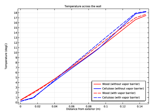
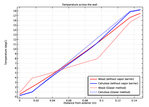
In the Settings window for 1D Plot Group, type Temperature across the wall (comparison) in the Label text field.
3
Locate the Data section. From the Dataset list, choose None.
4
Locate the Plot Settings section. Select the x-axis label check box.
5
In the associated text field, type Distance from exterior (m).
Wood (without vapor barrier)
1
Right-click Temperature across the wall (comparison) and choose Line Graph.
2
In the Settings window for Line Graph, locate the Data section.
3
From the Dataset list, choose Cut Line Wood (solution 1).
4
Locate the y-Axis Data section. From the Unit list, choose degC.
5
Click to expand the Coloring and Style section. From the Color list, choose Red.
6
In the Width text field, type 2.
7
Click to expand the Legends section. Select the Show legends check box.
8
From the Legends list, choose Manual.
9
10
In the Label text field, type Wood (without vapor barrier).
11
In the Temperature across the wall (comparison) toolbar, click  Plot.
Cellulose (without vapor barrier)
1
Right-click Wood (without vapor barrier) and choose Duplicate.
2
In the Settings window for Line Graph, type Cellulose (without vapor barrier) in the Label text field.
3
Locate the Data section. From the Dataset list, choose Cut Line Cellulose (solution 1).
4
Locate the Coloring and Style section. From the Color list, choose Blue.
5
Locate the Legends section. In the table, enter the following settings:
6
In the Temperature across the wall (comparison) toolbar, click  Plot.
Wood (with vapor barrier)
1
In the Model Builder window, right-click Wood (without vapor barrier) and choose Duplicate.
2
In the Settings window for Line Graph, type Wood (with vapor barrier) in the Label text field.
3
Locate the Data section. From the Dataset list, choose Cut Line Wood (solution 2) .
4
Locate the Coloring and Style section. Find the Line style subsection. From the Line list, choose Dashed.
5
Locate the Legends section. In the table, enter the following settings:
6
In the Temperature across the wall (comparison) toolbar, click  Plot.
Cellulose (with vapor barrier)
1
In the Model Builder window, right-click Cellulose (without vapor barrier) and choose Duplicate.
2
In the Settings window for Line Graph, type Cellulose (with vapor barrier) in the Label text field.
3
Locate the Data section. From the Dataset list, choose Cut Line Cellulose (solution 2) .
4
Locate the Coloring and Style section. Find the Line style subsection. From the Line list, choose Dashed.
5
Locate the Legends section. In the table, enter the following settings:
6
In the Temperature across the wall (comparison) toolbar, click  Plot.
Temperature across the wall (comparison)
1
In the Model Builder window, click Temperature across the wall (comparison).
2
In the Settings window for 1D Plot Group, locate the Legend section.
3
From the Position list, choose Lower right.
Wood (without vapor barrier)
1
In the Model Builder window, click Wood (without vapor barrier).
2
In the Settings window for Line Graph, click to expand the Title section.
3
From the Title type list, choose None.
Cellulose (without vapor barrier)
1
In the Model Builder window, click Cellulose (without vapor barrier).
2
In the Settings window for Line Graph, locate the Title section.
3
From the Title type list, choose None.
Wood (with vapor barrier)
1
In the Model Builder window, click Wood (with vapor barrier).
2
In the Settings window for Line Graph, locate the Title section.
3
From the Title type list, choose None.
Cellulose (with vapor barrier)
1
In the Model Builder window, click Cellulose (with vapor barrier).
2
In the Settings window for Line Graph, locate the Title section.
3
From the Title type list, choose None.
Temperature across the wall (comparison)
1
In the Model Builder window, click Temperature across the wall (comparison).
2
In the Settings window for 1D Plot Group, click to expand the Title section.
3
From the Title type list, choose Manual.
4
In the Title text area, type Temperature across the wall.
5
In the Temperature across the wall (comparison) toolbar, click  Plot.
Relative humidity across the wall (comparison)
1
Right-click Temperature across the wall (comparison) and choose Duplicate.
2
In the Model Builder window, click Temperature across the wall (comparison) 1.
3
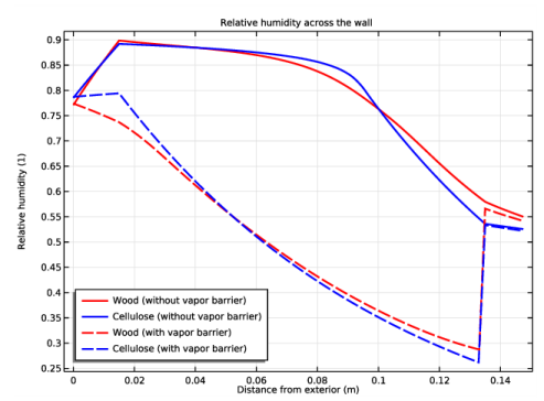
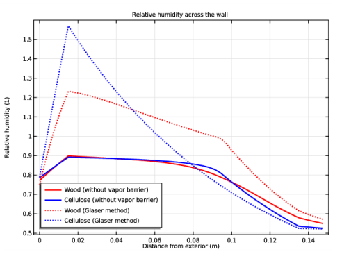
In the Settings window for 1D Plot Group, type Relative humidity across the wall (comparison) in the Label text field.
Wood (without vapor barrier)
1
In the Model Builder window, click Wood (without vapor barrier).
2
In the Settings window for Line Graph, locate the y-Axis Data section.
3
In the Expression text field, type mt.phi.
Cellulose (without vapor barrier)
1
In the Model Builder window, click Cellulose (without vapor barrier).
2
In the Settings window for Line Graph, locate the y-Axis Data section.
3
In the Expression text field, type mt.phi.
Wood (with vapor barrier)
1
In the Model Builder window, click Wood (with vapor barrier).
2
In the Settings window for Line Graph, locate the y-Axis Data section.
3
In the Expression text field, type mt.phi.
Cellulose (with vapor barrier)
1
In the Model Builder window, click Cellulose (with vapor barrier).
2
In the Settings window for Line Graph, locate the y-Axis Data section.
3
In the Expression text field, type mt.phi.
4
In the Relative humidity across the wall (comparison) toolbar, click  Plot.
Relative humidity across the wall (comparison)
1
In the Model Builder window, click Relative humidity across the wall (comparison).
2
In the Settings window for 1D Plot Group, locate the Legend section.
3
From the Position list, choose Lower left.
4
Locate the Title section. In the Title text area, type Relative humidity across the wall.
5
In the Relative humidity across the wall (comparison) toolbar, click  Plot.
Next, define new interfaces and a new study for the modeling of heat and moisture transport with the method described in Static modeling of Heat and Moisture Transport.
Add Physics
1
In the Home toolbar, click  Add Physics to open the Add Physics window.
2
Go to the Add Physics window.
3
In the tree, select Heat Transfer>Heat and Moisture Transport>Building Materials.
4
Click Add to Component 1 in the window toolbar.
Disable the multiphysics coupling node to be able to set the vapor permeability to 0 in the Heat Transfer in Building Materials interface. By doing this you ignore the latent heat effect in the heat transfer equation.
5
In the Home toolbar, click  Add Physics to close the Add Physics window.
Multiphysics
Heat and Moisture 2 (ham2)
In the Model Builder window, under Component 1 (comp1)>Multiphysics right-click Heat and Moisture 2 (ham2) and choose Disable.
Now, define the physics features.
Heat Transfer in Building Materials 2 (ht2)
Building Material 1
1
In the Model Builder window, under Component 1 (comp1)>Heat Transfer in Building Materials 2 (ht2) click Building Material 1.
2
In the Settings window for Building Material, locate the Model Inputs section.
3
From the φ list, choose Relative humidity (mt2/bm1).
4
Locate the Building Material Properties section. From the δp list, choose User defined. In the associated text field, type 0.
Heat Flux 1
1
In the Physics toolbar, click  Boundaries and choose Heat Flux.
2
In the Settings window for Heat Flux, locate the Heat Flux section.
3
Click the Convective heat flux button.
4
In the h text field, type h_ext.
5
In the Text text field, type T_ext.
6
Heat Flux 2
1
In the Physics toolbar, click  Boundaries and choose Heat Flux.
2
In the Settings window for Heat Flux, locate the Heat Flux section.
3
Click the Convective heat flux button.
4
In the h text field, type h_int.
5
In the Text text field, type T_int.
6
Initial Values 1
1
In the Model Builder window, click Initial Values 1.
2
In the Settings window for Initial Values, locate the Initial Values section.
3
In the T2 text field, type T_int.
Moisture Transport in Building Materials 2 (mt2)
Building Material 1
1
In the Model Builder window, under Component 1 (comp1)>Moisture Transport in Building Materials 2 (mt2) click Building Material 1.
2
In the Settings window for Building Material, locate the Model Input section.
3
From the T list, choose Temperature (ht2).
4
In the pA text field, type ht2.pA.
Set the moisture diffusivity to 0 to ignore the capillary transport of liquid moisture.
5
Locate the Building Material section. From the Dw list, choose User defined. From the Specify list, choose Vapor resistance factor.
Moisture Flux 1
1
In the Physics toolbar, click  Boundaries and choose Moisture Flux.
2
In the Settings window for Moisture Flux, locate the Moisture Flux section.
3
Click the Convective moisture flux, pressures difference button.
4
In the βp text field, type beta_ext.
5
In the Text text field, type T_ext.
6
In the φext text field, type phi_ext.
7
Moisture Flux 2
1
In the Physics toolbar, click  Boundaries and choose Moisture Flux.
2
In the Settings window for Moisture Flux, locate the Moisture Flux section.
3
Click the Convective moisture flux, pressures difference button.
4
In the βp text field, type beta_int.
5
In the Text text field, type T_int.
6
In the φext text field, type phi_int.
7
Initial Values 1
1
In the Model Builder window, click Initial Values 1.
2
In the Settings window for Initial Values, locate the Initial Values section.
3
In the φ0 text field, type phi_int.
Add Study
1
In the Home toolbar, click  Add Study to open the Add Study window.
2
Go to the Add Study window.
3
Find the Studies subsection. In the Select Study tree, select General Studies>Stationary.
4
Click Add Study in the window toolbar.
5
In the Home toolbar, click  Add Study to close the Add Study window.
Study 3
Step 1: Stationary
1
In the Settings window for Stationary, locate the Physics and Variables Selection section.
2
In the table, clear the Solve for check boxes for Heat Transfer in Building Materials (ht) and Moisture Transport in Building Materials (mt).
3
In the table, clear the Solve for check box for Heat and Moisture 1 (ham1).
4
In the Model Builder window, click Study 3.
5
In the Settings window for Study, type Study 3 (Stationary, Glaser method) in the Label text field.
6
In the Home toolbar, click  Compute.
Next, compare the results with those obtained with the first approach (without vapor barrier). Follow the instructions below to reproduce the plots of Figure 7 and Figure 8.
Results
Cut Line Wood (solution 2) 1
In the Model Builder window, right-click Cut Line Wood (solution 2) and choose Duplicate.
Cut Line Cellulose (solution 2) 1
In the Model Builder window, right-click Cut Line Cellulose (solution 2) and choose Duplicate.
Cut Line Wood (solution 3)
1
In the Settings window for Cut Line 2D, locate the Data section.
2
From the Dataset list, choose Study 3 (Stationary, Glaser method)/Solution 3 (sol3).
3
In the Label text field, type Cut Line Wood (solution 3) .
Cut Line Cellulose (solution 3)
1
In the Model Builder window, click Cut Line Cellulose (solution 2)  1.
2
In the Settings window for Cut Line 2D, locate the Data section.
3
From the Dataset list, choose Study 3 (Stationary, Glaser method)/Solution 3 (sol3).
4
In the Label text field, type Cut Line Cellulose (solution 3) .
Wood (with vapor barrier)
In the Model Builder window, right-click Wood (with vapor barrier) and choose Disable.
Cellulose (with vapor barrier)
In the Model Builder window, right-click Cellulose (with vapor barrier) and choose Disable.
Wood (without vapor barrier) 1
In the Model Builder window, right-click Wood (without vapor barrier) and choose Duplicate.
Cellulose (without vapor barrier) 1
In the Model Builder window, right-click Cellulose (without vapor barrier) and choose Duplicate.
Wood (Glaser method)
1
In the Settings window for Line Graph, type Wood (Glaser method) in the Label text field.
2
Locate the Data section. From the Dataset list, choose Cut Line Wood (solution 3) .
3
Locate the y-Axis Data section. In the Expression text field, type T2.
4
Locate the Coloring and Style section. Find the Line style subsection. From the Line list, choose Dotted.
5
Locate the Legends section. In the table, enter the following settings:
Cellulose (Glaser method)
1
In the Model Builder window, under Results>Temperature across the wall (comparison) click Cellulose (without vapor barrier)  1.
2
In the Settings window for Line Graph, type Cellulose (Glaser method) in the Label text field.
3
Locate the Data section. From the Dataset list, choose Cut Line Cellulose (solution 3) .
4
Locate the y-Axis Data section. In the Expression text field, type T2.
5
Locate the Coloring and Style section. Find the Line style subsection. From the Line list, choose Dotted.
6
Locate the Legends section. In the table, enter the following settings:
7
In the Temperature across the wall (comparison) toolbar, click  Plot.
Wood (with vapor barrier)
In the Model Builder window, right-click Wood (with vapor barrier) and choose Disable.
Cellulose (with vapor barrier)
In the Model Builder window, right-click Cellulose (with vapor barrier) and choose Disable.
Wood (without vapor barrier) 1
In the Model Builder window, right-click Wood (without vapor barrier) and choose Duplicate.
Cellulose (without vapor barrier) 1
In the Model Builder window, right-click Cellulose (without vapor barrier) and choose Duplicate.
Wood (Glaser method)
1
In the Settings window for Line Graph, type Wood (Glaser method) in the Label text field.
2
Locate the Data section. From the Dataset list, choose Cut Line Wood (solution 3) .
3
Locate the y-Axis Data section. In the Expression text field, type mt2.phi.
4
Locate the Coloring and Style section. Find the Line style subsection. From the Line list, choose Dotted.
5
Locate the Legends section. In the table, enter the following settings:
Cellulose (Glaser method)
1
In the Model Builder window, under Results>Relative humidity across the wall (comparison) click Cellulose (without vapor barrier)  1.
2
In the Settings window for Line Graph, type Cellulose (Glaser method) in the Label text field.
3
Locate the Data section. From the Dataset list, choose Cut Line Cellulose (solution 3) .
4
Locate the y-Axis Data section. In the Expression text field, type mt2.phi.
5
Locate the Coloring and Style section. Find the Line style subsection. From the Line list, choose Dotted.
6
Locate the Legends section. In the table, enter the following settings:
7
In the Relative humidity across the wall (comparison) toolbar, click  Plot.
Finally, use typical weather data for the temperature and relative humidity on exterior side, and set a new time-dependent study to check the evolution of the relative humidity in the bracing and in the isolation over two days. The weather data are available with the Heat Transfer Module license or the Subsurface Module license.
Definitions
Ambient Properties 1 (ampr1)
1
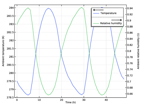
In the Model Builder window, under Component 1 (comp1)>Definitions>Shared Properties click Ambient Properties 1 (ampr1).
2
In the Settings window for Ambient Properties, locate the Ambient Settings section.
3
From the Ambient data list, choose Meteorological data (ASHRAE 2013).
4
Locate the Location section. Click Set Weather Station.
5
In the Weather Station dialog box, select Europe>Ireland>DUBLIN AIRPORT (039690) in the tree.
6
7
In the Settings window for Ambient Properties, locate the Time section.
8
Find the Date subsection. In the table, enter the following settings:
9
Find the Local time subsection. In the table, enter the following settings:
Add Study
1
In the Home toolbar, click  Add Study to open the Add Study window.
2
Go to the Add Study window.
3
Find the Studies subsection. In the Select Study tree, select General Studies>Time Dependent.
4
Click Add Study in the window toolbar.
5
In the Home toolbar, click  Add Study to close the Add Study window.
Study 4 (Time dependent, with vapor barrier)
1
In the Model Builder window, click Study 4.
2
In the Settings window for Study, type Study 4 (Time dependent, with vapor barrier) in the Label text field.
Step 1: Time Dependent
1
In the Model Builder window, under Study 4 (Time dependent, with vapor barrier) click Step 1: Time Dependent.
2
In the Settings window for Time Dependent, locate the Physics and Variables Selection section.
3
In the table, clear the Solve for check boxes for Heat Transfer in Building Materials 2 (ht2) and Moisture Transport in Building Materials 2 (mt2).
4
Locate the Study Settings section. From the Time unit list, choose h.
5
In the Output times text field, type range(0,1,48).
6
In the Home toolbar, click  Compute.
You can visualize the ambient data used as exterior conditions as in Figure 2 by following the instructions below.
Results
Ambient data
1
In the Home toolbar, click  Add Plot Group and choose 1D Plot Group.
2
In the Settings window for 1D Plot Group, type Ambient data in the Label text field.
3
Locate the Data section. From the Dataset list, choose Study 4 (Time dependent, with vapor barrier)/Solution 4 (sol4).
Point Graph 1
1
Right-click Ambient data and choose Point Graph.
2
3
In the Settings window for Point Graph, locate the y-Axis Data section.
4
In the Expression text field, type ampr1.T_amb.
5
Click to expand the Legends section. Select the Show legends check box.
6
From the Legends list, choose Manual.
7
Point Graph 2
1
In the Model Builder window, right-click Ambient data and choose Point Graph.
2
3
In the Settings window for Point Graph, locate the y-Axis Data section.
4
In the Expression text field, type ampr1.phi_amb.
5
Locate the Legends section. Select the Show legends check box.
6
From the Legends list, choose Manual.
7
Ambient data
1
In the Model Builder window, click Ambient data.
2
In the Settings window for 1D Plot Group, locate the Plot Settings section.
3
Select the Two y-axes check box.
4
In the table, select the Plot on secondary y-axis check box for Point Graph 2.
5
Locate the Title section. From the Title type list, choose None.
6
Click the  Zoom Extents button in the Graphics toolbar.
7
In the Ambient data toolbar, click  Plot.
Finally, define probes to plot the relative humidity in the bracing and in the isolation over time.
Definitions
Domain Point Probe: Relative humidity (bracing)
1
In the Definitions toolbar, click  Probes and choose Domain Point Probe.
2
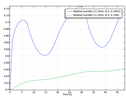
In the Settings window for Domain Point Probe, type Domain Point Probe: Relative humidity (bracing) in the Label text field.
3
Locate the Point Selection section. In row Coordinates, set x to L/2.
4
In row Coordinates, set y to t_il+t_i+t_b*0.95.
Point Probe Expression 1 (ppb1)
1
In the Model Builder window, expand the Domain Point Probe: Relative humidity (bracing) node, then click Point Probe Expression 1 (ppb1).
2
In the Settings window for Point Probe Expression, locate the Expression section.
3
In the Expression text field, type mt.phi.
4
Click  Update Results.
Domain Point Probe: Relative humidity (isolation)
1
In the Model Builder window, right-click Domain Point Probe: Relative humidity (bracing) and choose Duplicate.
2
In the Model Builder window, click Domain Point Probe: Relative humidity (bracing) 1.
3
In the Settings window for Domain Point Probe, type Domain Point Probe: Relative humidity (isolation) in the Label text field.
4
Locate the Point Selection section. In row Coordinates, set y to t_il+t_i*0.95.
Point Probe Expression 1 (ppb2)
1
In the Model Builder window, click Point Probe Expression 1 (ppb2).
2
In the Settings window for Point Probe Expression, click to expand the Table and Window Settings section.
3
From the Output table list, choose New table.
4
Click  Update Results.
Results
Relative humidity over two days
1
In the Model Builder window, under Results click Probe Plot Group 16.
2
In the Settings window for 1D Plot Group, type Relative humidity over two days in the Label text field.
3
In the Relative humidity over two days toolbar, click  Plot.
To create a 3D plot of the relative humidity, follow the instructions below.
Extrusion 2D 1
1
In the Results toolbar, click  More Datasets and choose Extrusion 2D.
2
In the Settings window for Extrusion 2D, locate the Data section.
3
From the Dataset list, choose Study 2 (Stationary, with vapor barrier)/Solution 2 (sol2).
4
Locate the Extrusion section. In the z maximum text field, type 0.2.
Relative humidity 3D
1
In the Results toolbar, click  3D Plot Group.
2
In the Settings window for 3D Plot Group, type Relative humidity 3D in the Label text field.
Relative humidity
1
Right-click Relative humidity 3D and choose Surface.
2
In the Settings window for Surface, type Relative humidity in the Label text field.
3
Locate the Expression section. In the Expression text field, type mt.phi.
4
In the Relative humidity 3D toolbar, click  Plot.