|
|
|

|
1
|
|
2
|
|
3
|
Click Add.
|
|
4
|
Click
|
|
5
|
|
6
|
Click
|
|
1
|
|
2
|
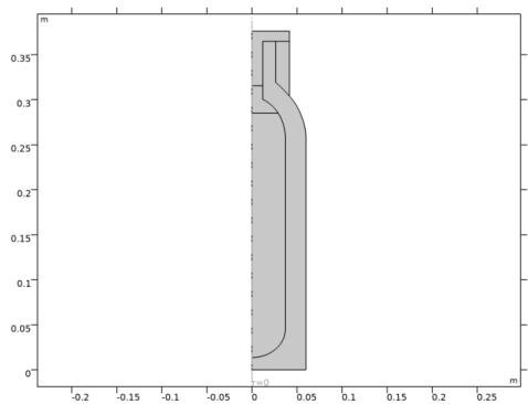
Browse to the model’s Application Libraries folder and double-click the file vacuum_flask_geom_sequence.mph.
|
|
3
|
|
4
|
|
1
|
|
2
|
|
3
|
|
1
|
|
2
|
|
3
|
|
1
|
|
2
|
|
1
|
|
2
|
|
3
|
In the tree, select Built-in>Air.
|
|
4
|
|
5
|
|
6
|
|
7
|
In the tree, select Built-in>Nylon.
|
|
8
|
|
9
|
|
10
|
|
11
|
|
1
|
|
1
|
|
1
|
|
2
|
|
3
|
|
4
|
|
5
|
Click to expand the Material Properties section. In the Material properties tree, select Geometric Properties>Shell>Thickness (lth).
|
|
6
|
|
7
|
Click to collapse the Material Properties section. Locate the Material Contents section. In the table, enter the following settings:
|
|
1
|
|
2
|
|
4
|
|
1
|
|
2
|
|
3
|
|
1
|
|
2
|
|
3
|
|
1
|
In the Model Builder window, under Component 1 (comp1)>Heat Transfer in Solids (ht) click Initial Values 1.
|
|
2
|
|
3
|
|
1
|
|
1
|
|
2
|
In the Settings window for Isothermal Domain Interface, locate the Isothermal Domain Interface section.
|
|
3
|
|
4
|
|
1
|
|
3
|
|
4
|
|
1
|
|
2
|
|
3
|
|
4
|
|
1
|
|
2
|
|
3
|
|
4
|
|
5
|
|
6
|
|
7
|
|
1
|
|
3
|
|
4
|
|
5
|
|
6
|
|
7
|
|
8
|
|
1
|
|
2
|
|
3
|
|
4
|
|
1
|
|
2
|
|
3
|
|
4
|
|
5
|
|
1
|
|
2
|
|
3
|
|
4
|
|
1
|
|
2
|
|
3
|
|
4
|
|
1
|
|
2
|
|
3
|
|
4
|
|
1
|
|
2
|
|
1
|
|
2
|
|
3
|
|
4
|
|
5
|
|
6
|
|
1
|
|
2
|
|
3
|
|
4
|
Find the Physics interfaces in study subsection. In the table, clear the Solve check box for Study 1.
|
|
5
|
|
6
|
|
1
|
|
2
|
|
3
|
|
4
|
Find the Physics interfaces in study subsection. In the table, clear the Solve check box for Heat Transfer in Solids (ht).
|
|
5
|
|
6
|
|
1
|
|
2
|
|
3
|
|
4
|
|
5
|
Click Import.
|
|
1
|
|
2
|
|
3
|
|
4
|
|
5
|
|
6
|
|
1
|
|
2
|
|
3
|
|
1
|
|
2
|
|
3
|
|
1
|
|
2
|
|
3
|
In the tree, select Built-in>Air.
|
|
4
|
|
5
|
|
6
|
|
7
|
In the tree, select Built-in>Nylon.
|
|
8
|
|
9
|
|
10
|
|
11
|
|
1
|
|
1
|
|
1
|
|
2
|
|
3
|
|
4
|
|
5
|
Click to expand the Material Properties section. In the Material properties tree, select Geometric Properties>Shell>Thickness (lth).
|
|
6
|
|
7
|
Click to collapse the Material Properties section. Locate the Material Contents section. In the table, enter the following settings:
|
|
1
|
|
2
|
|
4
|
|
1
|
|
3
|
|
4
|
|
5
|
|
6
|
|
7
|
Click OK.
|
|
1
|
|
2
|
|
3
|
|
1
|
In the Model Builder window, under Component 2 (comp2) click Heat Transfer in Solids and Fluids 2 (ht2).
|
|
2
|
|
3
|
|
1
|
In the Model Builder window, under Component 2 (comp2)>Heat Transfer in Solids and Fluids 2 (ht2) click Fluid 1.
|
|
2
|
|
3
|
|
1
|
|
2
|
|
3
|
|
1
|
|
1
|
In the Model Builder window, under Component 2 (comp2) click Heat Transfer in Solids and Fluids 2 (ht2).
|
|
2
|
|
3
|
|
1
|
|
1
|
|
2
|
In the Settings window for Isothermal Domain Interface, locate the Isothermal Domain Interface section.
|
|
3
|
|
4
|
|
1
|
|
3
|
|
4
|
|
1
|
|
2
|
|
3
|
|
4
|
|
1
|
|
3
|
|
4
|
|
1
|
|
2
|
|
3
|
|
4
|
|
1
|
|
2
|
|
3
|
|
4
|
|
1
|
|
2
|
|
3
|
|
4
|
|
5
|
|
1
|
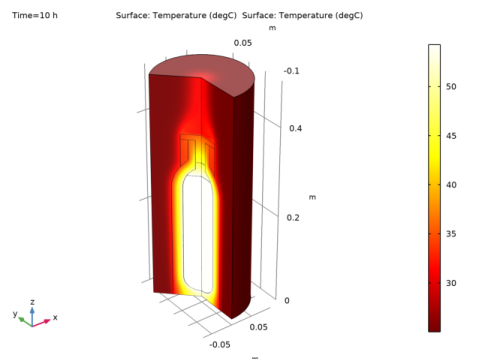
In the Model Builder window, under Results, Ctrl-click to select Temperature, 3D (ht), Isothermal Contours (ht), and Shell Temperature, 3D (ht).
|
|
2
|
Right-click and choose Group.
|
|
1
|
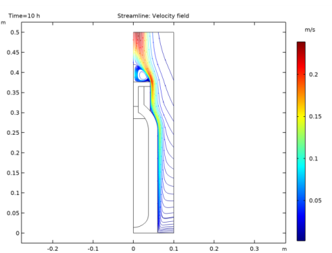
In the Model Builder window, under Results, Ctrl-click to select Temperature, 3D (ht2), Isothermal Contours (ht2), Velocity (spf), Pressure (spf), and Velocity, 3D (spf).
|
|
2
|
Right-click and choose Group.
|
|
1
|
|
2
|
|
3
|
|
1
|
|
2
|
|
3
|
|
4
|
|
5
|
|
1
|
|
2
|
|
1
|
|
2
|
|
3
|
|
4
|
|
5
|
|
6
|
|
1
|
|
2
|
|
3
|
|
4
|
|
5
|
|
1
|
|
2
|
In the Settings window for Streamline, click Replace Expression in the upper-right corner of the Expression section. From the menu, choose Component 2 (comp2)>Laminar Flow>Velocity and pressure>u,w - Velocity field.
|
|
3
|
|
4
|
Locate the Coloring and Style section. Find the Point style subsection. From the Type list, choose Arrow.
|
|
1
|
|
2
|
In the Settings window for Color Expression, click Replace Expression in the upper-right corner of the Expression section. From the menu, choose Component 2 (comp2)>Laminar Flow>Velocity and pressure>spf.U - Velocity magnitude - m/s.
|
|
3
|
|
4
|
|
1
|
|
2
|
|
1
|
|
2
|
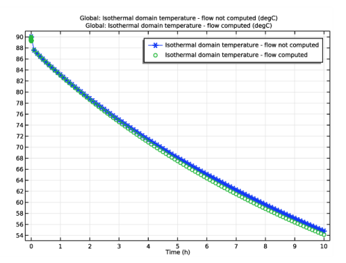
In the Settings window for Global, click Replace Expression in the upper-right corner of the y-Axis Data section. From the menu, choose Component 1 (comp1)>Heat Transfer in Solids>Temperature>ht.id1.T - Isothermal domain temperature - K.
|
|
3
|
|
4
|
Click to expand the Coloring and Style section. Find the Line markers subsection. From the Marker list, choose Cycle.
|
|
5
|
|
1
|
|
2
|
|
3
|
|
4
|
Click Replace Expression in the upper-right corner of the y-Axis Data section. From the menu, choose Component 2 (comp2)>Heat Transfer in Solids and Fluids 2>Temperature>ht2.id1.T - Isothermal domain temperature - K.
|
|
5
|
|
6
|
Locate the Coloring and Style section. Find the Line style subsection. From the Line list, choose None.
|
|
7
|
|
8
|
|
9
|
|
1
|
|
2
|
|
3
|
|
4
|
|
1
|
|
2
|
|
3
|
|
4
|
|
5
|
|
6
|
|
7
|
|
8
|
|
1
|
|
2
|
|
3
|
|
4
|
|
5
|
|
6
|
|
7
|
|
8
|
|
9
|
|
10
|
|
1
|
|
2
|
|
1
|
|
2
|
|
1
|
|
2
|
|
3
|
|
4
|
|
5
|
|
6
|
|
1
|
|
2
|
|
3
|
|
4
|
|
5
|
|
6
|
|
1
|
|
2
|
|
3
|
|
4
|
|
5
|
|
6
|
|
7
|
|
8
|
|
1
|
|
2
|
|
3
|
|
4
|
|
5
|
|
6
|
|
7
|
|
8
|
|
1
|
|
2
|
|
3
|
|
4
|
|
5
|
In the r text field, type 0.66*radius 0.66*radius 0.66*radius 0.3*radius 0.3*radius 0.3*radius 0.3*radius 0.3*radius.
|
|
6
|
In the z text field, type 0.84*height 0.96*height 0.96*height 0.96*height 0.96*height 0.83*height 0.83*height 0.79*height.
|
|
1
|
|
2
|
|
3
|
|
4
|
|
5
|
|
6
|
|
7
|
|
8
|
|
1
|
|
2
|
|
3
|
|
4
|
|
5
|
|
6
|
|
7
|
|
8
|
|
1
|
|
2
|
|
3
|
|
4
|
|
5
|
|
6
|
|
7
|
|
8
|
|
1
|
|
2
|
|
3
|
|
4
|
|
5
|
|
6
|
|
7
|
|
8
|
|
1
|
|
2
|
|
3
|
|
4
|
On the object pol1, select Point 1 only.
|
|
5
|
Locate the Endpoint section. Find the End vertex subsection. Select the
|
|
6
|
On the object qb5, select Point 2 only.
|
|
7
|
|
1
|
|
2
|
|
1
|
|
2
|
Click in the Graphics window and then press Ctrl+A to select both objects.
|
|
1
|
|
2
|
|
3
|
|
4
|
|
5
|
|
6
|
|
7
|
|
8
|
|
1
|
|
2
|
|
3
|
|
4
|
|
5
|
|
6
|
Locate the Endpoint section. Find the End vertex subsection. Select the
|
|
7
|
On the object csol2, select Point 9 only.
|
|
1
|
|
2
|
|
3
|
|
4
|
|
5
|
|
1
|
|
2
|
On the object fin, select Boundaries 9 and 17 only.
|
|
3
|