|
|
|
|
ρ0
|
||
|
αp
|
||
|
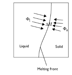
ΔH
|
|
1
|
|
2
|
|
3
|
Click Add.
|
|
4
|
Click
|
|
5
|
|
6
|
Click
|
|
1
|
|
2
|
|
1
|
|
2
|
|
3
|
|
4
|
Click to expand the Layers section. In the table, enter the following settings:
|
|
5
|
|
6
|
|
7
|
|
1
|
|
2
|
|
1
|
|
1
|
In the Model Builder window, under Component 1 (comp1) click Heat Transfer in Solids and Fluids (ht).
|
|
2
|
|
3
|
|
1
|
In the Model Builder window, under Component 1 (comp1)>Heat Transfer in Solids and Fluids (ht) click Fluid 1.
|
|
1
|
|
2
|
|
1
|
|
2
|
|
3
|
|
4
|
Click OK.
|
|
6
|
|
1
|
In the Model Builder window, under Component 1 (comp1)>Heat Transfer in Solids and Fluids (ht) click Initial Values 1.
|
|
2
|
|
3
|
|
1
|
|
2
|
|
3
|
|
4
|
|
5
|
|
1
|
|
3
|
|
4
|
|
1
|
|
3
|
|
4
|
|
1
|
|
3
|
|
4
|
|
5
|
|
6
|
|
1
|
|
1
|
In the Model Builder window, under Component 1 (comp1)>Multiphysics click Nonisothermal Flow 1 (nitf1).
|
|
2
|
|
3
|
|
4
|
|
5
|
|
6
|
|
1
|
|
2
|
|
3
|
|
4
|
|
1
|
|
1
|
|
2
|
|
3
|
|
4
|
|
1
|
|
2
|
|
3
|
Click
|
|
4
|
|
5
|
|
6
|
Click Replace.
|
|
7
|
|
8
|
|
9
|
|
1
|
|
2
|
|
3
|
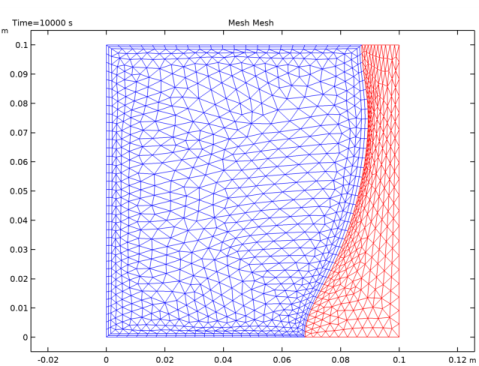
In the Model Builder window, expand the Study 1>Solver Configurations>Solution 1 (sol1)>Dependent Variables 1 node, then click Material mesh displacement (comp1.material.disp).
|
|
4
|
|
5
|
|
6
|
|
1
|
|
2
|
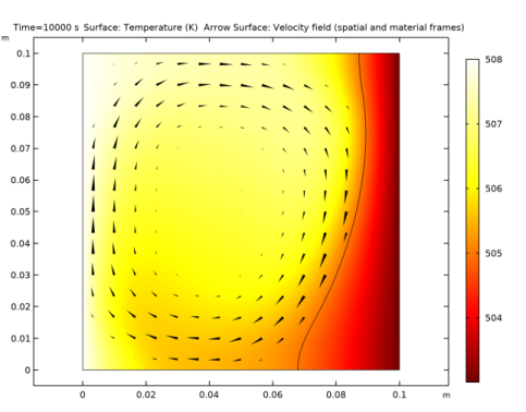
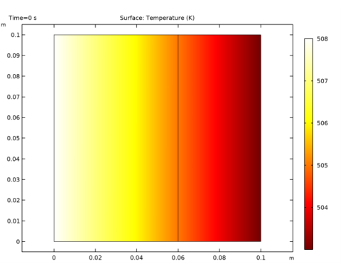
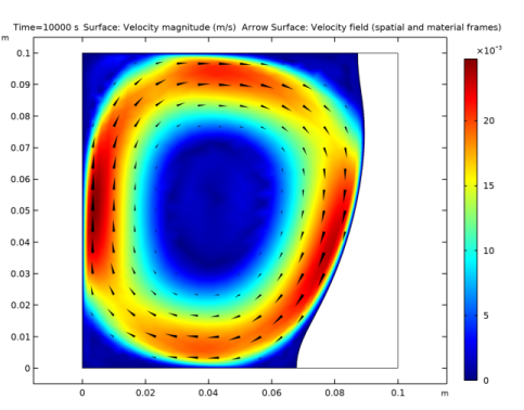
In the Settings window for Arrow Surface, click Replace Expression in the upper-right corner of the Expression section. From the menu, choose Component 1 (comp1)>Laminar Flow>Velocity and pressure>u,v - Velocity field (spatial and material frames).
|
|
3
|
|
4
|
|
5
|
|
1
|
|
1
|
|
2
|
In the Settings window for Arrow Surface, click Replace Expression in the upper-right corner of the Expression section. From the menu, choose Component 1 (comp1)>Laminar Flow>Velocity and pressure>u,v - Velocity field (spatial and material frames).
|
|
3
|
|
4
|
|
5
|
|
1
|
|
2
|
|
1
|
|
2
|
|
3
|
|
4
|
|
1
|
|
2
|
|
3
|
|
4
|
|
1
|
In the Model Builder window, under Results>Mesh Deformation right-click Mesh 1 and choose Duplicate.
|
|
2
|
|
3
|
|
1
|
|
2
|
|
3
|
|
4
|