PDF

Thermoelectric Leg
Introduction
A thermocouple is made of two different conductors (legs) in contact with each other at one point (junction). When a temperature difference is established between the two legs, then a voltage is established across the junction. Therefore a thermocouple properly calibrated is a temperature sensor and can convert temperature gradients into electric currents. In this validation example, we verify the response of one leg when a current is passed through the device. A cooling effect, known as the Peltier effect, is expected.
Model Definition
The component is 1-by-1-by-6 mm, as shown in Figure 1. The core of the device, the thermoelectric part, is made of bismuth telluride (Bi2Te3). It is capped by two thin copper electrodes, 0.1 mm thick.
Figure 1: Thermoelectric leg geometry.
The material properties are available in COMSOL Multiphysics Material Library. However, since the properties for bismuth telluride slightly differ from these from the original benchmark, values from Ref. 1 are used in this application.
Table 1: Material properties for Bismuth Telluride.
In addition Seebeck coefficient for copper, 6.5·10-6 V/K, is also taken from Ref. 1.
The bottom electrode surface is held at 0°C while the top electrode and the lateral surfaces are thermally insulated.
The bottom electrode is electrically grounded at 0 V. The total inward electric current through the top electrode is 0.7 A. The lateral surfaces are electrically insulated.
Results and Discussion
The current circulating in the thermoelectric device is responsible for the cooling effect shown in Figure 2. The temperature field is in complete agreement with the results from Ref. 1.
Figure 2: Temperature field on the thermoelectric leg surface.
Figure 3 shows the isothermal surfaces and the heat flux which is in the same direction as the electric current (from the top to the bottom).
Figure 3: Isothermal surfaces and heat flux in the thermoelectric leg.
The top level electrode reaches an electric potential of around 49.1 mV due to the inward current density set on this boundary. This corresponds to the value presented in Ref. 1.
Figure 4: Electric potential in the thermoelectric leg.
Reference
1. M. Jaegle, Multiphysics Simulation of Thermoelectric Systems, “Modeling of Peltier-Cooling and Thermoelectric Generation,” Proc. COMSOL Conf. 2008 Hanover, 2008.
Application Library path: Heat_Transfer_Module/Verification_Examples/thermoelectric_leg
Modeling Instructions
From the File menu, choose New.
New
In the New window, click  Model Wizard.
Model Wizard
1
In the Model Wizard window, click  3D.
2
In the Select Physics tree, select Heat Transfer>Thermoelectric Effect.
3
Click Add.
4
Click  Study.
5
In the Select Study tree, select General Studies>Stationary.
6
Geometry 1
1
In the Model Builder window, under Component 1 (comp1) click Geometry 1.
2
In the Settings window for Geometry, locate the Units section.
3
From the Length unit list, choose mm.
Block 1 (blk1)
1
In the Geometry toolbar, click  Block.
2
In the Settings window for Block, locate the Size and Shape section.
3
In the Height text field, type 6.
4
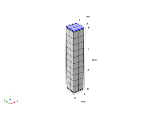
Click to expand the Layers section. In the table, enter the following settings:
5
Find the Layer position subsection. Select the Top check box.
6
Click  Build All Objects.
7
Click the  Zoom Extents button in the Graphics toolbar.
Now define the parameters that will be used for the model. The inward current density, J0, corresponds to a total current of 0.7 A through a 1x1 mm square.
Global Definitions
Parameters 1
1
In the Model Builder window, under Global Definitions click Parameters 1.
2
In the Settings window for Parameters, locate the Parameters section.
3
Materials
Bismuth Telluride - Bi2Te3
1
In the Materials toolbar, click  Blank Material.
2
In the Settings window for Material, type Bismuth Telluride - Bi2Te3 in the Label text field.
3
Locate the Material Contents section. In the table, enter the following settings:
Add Material
1
In the Materials toolbar, click  Add Material to open the Add Material window.
2
Go to the Add Material window.
3
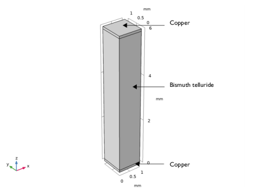
In the tree, select Built-in>Copper.
4
Click Add to Component in the window toolbar.
5
In the Materials toolbar, click  Add Material to close the Add Material window.
Materials
Copper (mat2)
1
2
In the Settings window for Material, locate the Material Contents section.
3
Heat Transfer in Solids (ht)
Temperature 1
1
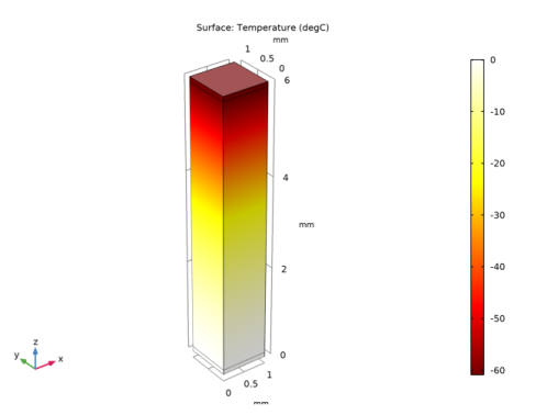
In the Model Builder window, under Component 1 (comp1) right-click Heat Transfer in Solids (ht) and choose Temperature.
2
Click the  Wireframe Rendering button in the Graphics toolbar.
3
4
In the Settings window for Temperature, locate the Temperature section.
5
In the T0 text field, type T0.
Electric Currents (ec)
In the Model Builder window, under Component 1 (comp1) click Electric Currents (ec).
Ground 1
1
In the Physics toolbar, click  Boundaries and choose Ground.
2
Normal Current Density 1
1
In the Physics toolbar, click  Boundaries and choose Normal Current Density.
2
3
In the Settings window for Normal Current Density, locate the Normal Current Density section.
4
In the Jn text field, type J0.
Due to the geometrical properties, replacing the default tetrahedral mesh by a hexahedral sweep mesh is more suited.
Mesh 1
Swept 1
1
In the Mesh toolbar, click  Swept.
2
In the Settings window for Swept, click to expand the Source Faces section.
3
Now visualize the mesh and compare it with the figure below.
4
Click  Build All.
Study 1
In the Home toolbar, click  Compute.
Results
Temperature (ht)
The first default plot shows the temperature field; compare with Figure 2.
Surface
1
In the Model Builder window, expand the Temperature (ht) node, then click Surface.
2
In the Settings window for Surface, locate the Expression section.
3
From the Unit list, choose degC.
4
In the Temperature (ht) toolbar, click  Plot.
Isothermal Contours (ht)
The second default plot shows the isothermal surfaces. Change the unit to Celsius degrees and add the heat flux to obtain a figure similar to Figure 3.
Isosurface
1
In the Model Builder window, expand the Isothermal Contours (ht) node, then click Isosurface.
2
In the Settings window for Isosurface, locate the Expression section.
3
From the Unit list, choose degC.
Arrow Volume 1
1
In the Model Builder window, right-click Isothermal Contours (ht) and choose Arrow Volume.
2
In the Settings window for Arrow Volume, locate the Arrow Positioning section.
3
Find the X grid points subsection. In the Points text field, type 2.
4
Find the Y grid points subsection. In the Points text field, type 2.
5
Locate the Coloring and Style section. From the Arrow length list, choose Logarithmic.
6
In the Isothermal Contours (ht) toolbar, click  Plot.
Electric Potential (ec)
The third default plot group shows the electric potential distribution as in Figure 4.