PDF

Rapid Thermal Annealing
Introduction
In the semiconductor industry, rapid thermal annealing (RTA) is a semiconductor process step used for the activation of dopants and the interfacial reaction of metal contacts. In principle, the operation involves rapid heating of a wafer from ambient to approximately 10001500 K. As soon as the wafer reaches this temperature, it is held there for a few seconds and then finally quenched. A rapid process step is crucial to avoid too much diffusion of the dopants. Furthermore, it is also important to avoid overheating and nonuniform temperature distributions to occur. An RTA apparatus, schematically shown in Figure 1, uses high-power IR lamps as heat sources (Ref. 1).
Figure 1: Diagram of a typical RTA (rapid thermal annealing) apparatus.
A technical difficulty lies in how to properly measure the wafer’s temperature during the process. Two commonly used technical solutions are: thermocouples and IR sensors.
To achieve an accurate measurement, it is important that the temperature sensor not be subjected to direct radiation from the lamp. Ideally positioned, the sensor only receives secondary radiation; that is, the radiation reflected and emitted by the silicon wafer. Desirable characteristics of the sensor are high accuracy and short response time. While a high-performance design requires superior electronics, the sensor geometry plays a big role. In a nutshell, the sensor needs to be large enough to register a sufficient amount of radiation but light enough to minimize its own thermal inertia. Since COMSOL Multiphysics gives you control over the geometry, a parameter optimization of the sensor could be an exciting project. But first, justify that an infrared sensor is indeed more appropriate than the inexpensive thermocouple.
Model Definition
Figure 1 illustrates a typical RTA configuration. In many applications, RTA makes use of double-sided heating, in which IR lamps are positioned both above and below the silicon wafer. In this example we are modeling a single-sided heating apparatus, as shown in Figure 2.
Figure 2: The model geometry.
The components in Figure 2 are contained in a chamber with temperature-controlled walls with a set point of 400 K. This results in a closed cavity so you can omit the geometry of the chamber walls. Furthermore, the model assumes that this physical system is dominated by radiation and convection cooling. The convective cooling of the wafer and sensor to the gas (at 400 K) is modeled using a heat transfer coefficient, h (in this example set to 20 W/(m2·K)).
The problem is governed by the heat equation, given below together with its boundary conditions:
Here ρ is the density; k denotes the thermal conductivity; Q represents the volume heat source; n is the surface normal vector; Tinf equals the temperature of the convection cooling gas; ε denotes the surface emissivity; J0 is the expression for surface radiosity (further described in the Heat Transfer Module User’s Guide); and σ is the Stefan-Boltzmann constant.
The model simulates the lamp as a solid object with a volume heat source of 25 kW. It is insulated on all surfaces except the for the top, which faces the silicon wafer. At this surface, heat leaves the lamp as radiation only. In order to capture the lamp’s transient startup time, the model uses a low heat capacity, Cp, for the solid (10 J/(kg·K)). The lamp’s other thermal properties are identical to those of copper metal (the default value in the interface).
In this case assume that the wafer dissipates energy via radiation and convection on all surfaces. The sensor is insulated at all surfaces except the top, which is subjected to both convection and radiation. The thermal material properties are set to those of alumina.
The following table summarizes the material properties used in the application:
k (W/(m·K)) 
ρ (kg/m3) 
Cp (J/(kg·K))
ε
The model simulates the transient temperature field for 10 s of heating. The initial temperature is 400 K for all objects.
Results and Discussion
Figure 3 displays the temperature distribution after 10 s of heating.
Figure 3: Temperatures of the lamp, wafer, and sensor after 10 s of heating.
After 10 seconds, the temperatures of the wafer and sensor differ significantly: the wafer is close to 2000 K, whereas the sensor is close to 1200 K.
Notice that the temperature distribution in the wafer with a delta of several hundred degrees is not very uniform, and that you probably can do much better by reconfiguring the heat source. However, such a reconfiguration is not included in this application.
To investigate how well the sensor’s temperature reflects that of the wafer surface, it is useful to plot the temperature transient of the wafer surface’s centerpoint that faces the lamp (Twafer), together with the temperature at a point on the sensor top surface (Tsensor) (see Figure 4).
Figure 4: The temperature transients of the lamp, the silicon wafer, and the sensor, together with the irradiation power at the sensor surface.
The sensor temperature reflects that of the silicon wafer poorly. This means that the signal of a thermocouple, positioned anywhere in the sensor domain of Figure 2, is of little use for regulating this process.
The IR-detector transient (Sensirrad) matches the wafer temperature characteristic quite well. A scalar amplification allows for a high accuracy measurement of the wafer temperature. The precise amplification factor is system-dependent and subject to a calibration requirement.
However, IR-sensor methodology also has drawbacks. The IR signal depends on the emissivity of the wafer, which varies with temperature making the response nonlinear. Furthermore, the IR signal is very sensitive to geometry changes.
The bright side is that COMSOL Multiphysics does not set any limits with respect to these phenomena and allows you to study them fully.
Reference
1. A.T. Fiory, “Methods in Rapid Thermal Annealing,” Proc. 8th Int’l Conf. Advanced Thermal Processing of Semiconductors (RTP 2000).
Application Library path: Heat_Transfer_Module/Thermal_Radiation/thermal_annealing
Modeling Instructions
From the File menu, choose New.
New
In the New window, click  Model Wizard.
Model Wizard
1
In the Model Wizard window, click  3D.
2
In the Select Physics tree, select Heat Transfer>Radiation>Heat Transfer with Surface-to-Surface Radiation.
3
Click Add.
4
Click  Study.
5
In the Select Study tree, select General Studies>Time Dependent.
6
Global Definitions
Parameters 1
1
In the Model Builder window, under Global Definitions click Parameters 1.
2
In the Settings window for Parameters, locate the Parameters section.
3
Component 1 (comp1)
Set the geometric shape order to "Quadratic". By default, the geometric shape order is only linear in this model. Although the difference will not be visible when plotting the mesh (for graphics performance purposes), second-order elements will then be allowed, yielding a much better match between the mesh and the real cylindrical geometry thanks to the curved edges of the boundary elements.
1
In the Model Builder window, click Component 1 (comp1).
2
In the Settings window for Component, locate the General section.
3
Find the Mesh frame coordinates subsection. From the Geometry shape function list, choose Quadratic Lagrange.
Geometry 1
Cylinder 1 (cyl1)
1
In the Geometry toolbar, click  Cylinder.
2
In the Settings window for Cylinder, locate the Size and Shape section.
3
In the Radius text field, type 0.05.
4
In the Height text field, type 5e-4.
5
Click  Build Selected.
Cylinder 2 (cyl2)
1
In the Geometry toolbar, click  Cylinder.
2
In the Settings window for Cylinder, locate the Size and Shape section.
3
In the Radius text field, type 0.05.
4
In the Height text field, type 1e-3.
5
Locate the Position section. In the z text field, type -5e-2.
6
Click  Build Selected.
Cylinder 3 (cyl3)
1
In the Geometry toolbar, click  Cylinder.
2
In the Settings window for Cylinder, locate the Size and Shape section.
3
In the Radius text field, type 0.01.
4
In the Height text field, type 1e-3.
5
Locate the Position section. In the x text field, type 0.07.
6
In the z text field, type -5e-2.
7
Click  Build Selected.
8
Click the  Zoom Extents button in the Graphics toolbar.
The built geometry shows a plane symmetry. Delete half of it to optimize the computation.
Block 1 (blk1)
1
In the Geometry toolbar, click  Block.
2
In the Settings window for Block, locate the Size and Shape section.
3
In the Width text field, type 0.2.
4
In the Depth text field, type 0.2.
5
In the Height text field, type 0.2.
6
Locate the Position section. In the x text field, type -0.1.
7
In the y text field, type -0.2.
8
In the z text field, type -0.1.
9
Click  Build Selected.
Difference 1 (dif1)
1
In the Geometry toolbar, click  Booleans and Partitions and choose Difference.
2
Select the objects cyl1, cyl2, and cyl3 only.
3
In the Settings window for Difference, locate the Difference section.
4
Find the Objects to subtract subsection. Select the  Activate Selection toggle button.
5
6
Click  Build Selected.
7
In the Geometry toolbar, click  Build All.
8
Click the  Zoom Extents button in the Graphics toolbar.
In preparation for analyzing and visualizing the results, define a nonlocal integration coupling.
Definitions
Integration 1 (intop1)
1
In the Definitions toolbar, click  Nonlocal Couplings and choose Integration.
2
In the Settings window for Integration, locate the Source Selection section.
3
From the Geometric entity level list, choose Boundary.
4
Variables 1
1
In the Definitions toolbar, click  Local Variables.
2
In the Settings window for Variables, locate the Variables section.
3
ht.G_rad is a predefined physics interface variable representing inward radiation, which includes both surface-to-surface and surface-to-ambient contributions.
The integral is multiplied by 2 to get the irradiated heat effect on the full geometry.
Materials
IR Lamp
1
In the Materials toolbar, click  Blank Material.
2
In the Settings window for Material, type IR Lamp in the Label text field.
3
4
Locate the Material Contents section. In the table, enter the following settings:
Add Material
1
In the Materials toolbar, click  Add Material to open the Add Material window.
2
Go to the Add Material window.
3
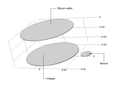
In the tree, select Built-in>Silicon.
4
Click Add to Component in the window toolbar.
5
In the Materials toolbar, click  Add Material to close the Add Material window.
Materials
Silicon (mat2)
Select Domain 2 only.
Sensor
1
In the Materials toolbar, click  Blank Material.
2
In the Settings window for Material, type Sensor in the Label text field.
3
4
Locate the Material Contents section. In the table, enter the following settings:
Now add materials on the boundaries for the specification of surface emissivities.
IR Lamp (Boundaries)
1
In the Model Builder window, under Component 1 (comp1)>Materials right-click IR Lamp (mat1) and choose Duplicate.
2
In the Settings window for Material, type IR Lamp (Boundaries) in the Label text field.
3
Locate the Geometric Entity Selection section. From the Geometric entity level list, choose Boundary.
4
5
Click to expand the Material Properties section. In the Material properties tree, select Basic Properties>Surface Emissivity.
6
Click  Add to Material.
7
Locate the Material Contents section. In the table, enter the following settings:
Silicon (Boundaries)
1
In the Model Builder window, under Component 1 (comp1)>Materials right-click Silicon (mat2) and choose Duplicate.
2
In the Settings window for Material, type Silicon (Boundaries) in the Label text field.
3
Locate the Geometric Entity Selection section. From the Geometric entity level list, choose Boundary.
4
5
Click to expand the Material Properties section. In the Material properties tree, select Basic Properties>Surface Emissivity.
6
Click  Add to Material.
7
Locate the Material Contents section. In the table, enter the following settings:
Sensor (Boundaries)
1
In the Model Builder window, under Component 1 (comp1)>Materials right-click Sensor (mat3) and choose Duplicate.
2
In the Settings window for Material, type Sensor (Boundaries) in the Label text field.
3
Locate the Geometric Entity Selection section. From the Geometric entity level list, choose Boundary.
4
5
Click to expand the Material Properties section. In the Material properties tree, select Basic Properties>Surface Emissivity.
6
Click  Add to Material.
7
Locate the Material Contents section. In the table, enter the following settings:
Heat Transfer in Solids (ht)
Heat Source 1
1
In the Model Builder window, under Component 1 (comp1) right-click Heat Transfer in Solids (ht) and choose Heat Source.
2
3
In the Settings window for Heat Source, locate the Heat Source section.
4
Click the Heat rate button.
Define the total power as half of the lamp power on the reduced geometry.
5
In the P0 text field, type P_lamp/2.
Initial Values 1
1
In the Model Builder window, click Initial Values 1.
2
In the Settings window for Initial Values, locate the Initial Values section.
3
In the T text field, type T_wall.
Heat Flux 1
1
In the Physics toolbar, click  Boundaries and choose Heat Flux.
2
3
In the Settings window for Heat Flux, locate the Heat Flux section.
4
Click the Convective heat flux button.
5
In the h text field, type h_gas.
6
In the Text text field, type T_gas.
Symmetry 1
1
In the Physics toolbar, click  Boundaries and choose Symmetry.
2
With the Symmetry feature, only the symmetry of the temperature field is handled. To consider also symmetry for radiation computation, add a Symmetry for Surface-to-Surface Radiation feature.
Surface-to-Surface Radiation (rad)
1
In the Model Builder window, under Component 1 (comp1) click Surface-to-Surface Radiation (rad).
2
Diffuse Surface 1
1
In the Model Builder window, under Component 1 (comp1)>Surface-to-Surface Radiation (rad) click Diffuse Surface 1.
2
In the Settings window for Diffuse Surface, locate the Ambient section.
3
Find the Ambient temperature subsection. In the Tamb text field, type T_wall.
By default the radiation direction is controlled by the opacity of the domains. The solid parts are automatically defined as opaque. You can change this setting by modifying the Opacity subnode under the Solid feature.
Symmetry for Surface-to-Surface Radiation 1
1
In the Physics toolbar, click  Global and choose Symmetry for Surface-to-Surface Radiation.
2
In the Settings window for Symmetry for Surface-to-Surface Radiation, locate the Plane Symmetry section.
3
From the Selection method list, choose Point selection.
4
Locate the First Point Defining Reflection Plane section. Select the  Activate Selection toggle button.
5
6
Locate the Second Point Defining Reflection Plane section. Select the  Activate Selection toggle button.
7
8
Locate the Third Point Defining Reflection Plane section. Select the  Activate Selection toggle button.
9
Mesh 1
Free Triangular 1
In the Mesh toolbar, click  Boundary and choose Free Triangular.
Size
1
In the Model Builder window, click Size.
2
In the Settings window for Size, locate the Element Size section.
3
From the Predefined list, choose Finer.
Free Triangular 1
1
In the Model Builder window, click Free Triangular 1.
2
Swept 1
1
In the Mesh toolbar, click  Swept.
2
In the Settings window for Swept, click  Build All.
Study 1
Step 1: Time Dependent
1
In the Model Builder window, under Study 1 click Step 1: Time Dependent.
2
In the Settings window for Time Dependent, locate the Study Settings section.
3
In the Output times text field, type 0 10.
4
From the Tolerance list, choose User controlled.
5
In the Relative tolerance text field, type 1e-3.
Solution 1 (sol1)
1
In the Study toolbar, click  Show Default Solver.
2
In the Model Builder window, expand the Solution 1 (sol1) node, then click Time-Dependent Solver 1.
3
In the Settings window for Time-Dependent Solver, click to expand the Output section.
4
Locate the General section. From the Times to store list, choose Steps taken by solver.
5
In the Study toolbar, click  Compute.
Results
Temperature (ht)
1
In the Temperature (ht) toolbar, click  Plot.
2
Click the  Zoom Extents button in the Graphics toolbar.
The first default 3D plot shows the temperature at the final time step on half of the full geometry. To visualize the temperature on the full geometry, define a new dataset.
Mirror 3D 1
1
In the Results toolbar, click  More Datasets and choose Mirror 3D.
2
In the Settings window for Mirror 3D, locate the Plane Data section.
3
From the Plane list, choose ZX-planes.
4
Temperature (ht)
1
In the Model Builder window, click Temperature (ht).
2
In the Settings window for 3D Plot Group, locate the Data section.
3
From the Dataset list, choose Mirror 3D 1.
4
In the Temperature (ht) toolbar, click  Plot.
5
Click the  Zoom Extents button in the Graphics toolbar.
You can now see the plot of Figure 3.
Two other default plots show isothermal contours and radiosity.
Reproduce the plots in Figure 4 with the following steps:
Cut Point 3D 1
1
In the Results toolbar, click  Cut Point 3D.
2
In the Settings window for Cut Point 3D, locate the Point Data section.
3
In the X text field, type 0, 0, 0.06.
4
In the Y text field, type 0.
5
In the Z text field, type -0.049, 0, -0.049.
Temperature and Signal Transients
1
In the Results toolbar, click  1D Plot Group.
2
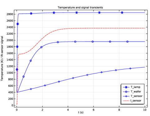
In the Settings window for 1D Plot Group, type Temperature and Signal Transients in the Label text field.
3
Click to expand the Title section. From the Title type list, choose Manual.
4
In the Title text area, type Temperature and signal transients.
5
Locate the Plot Settings section. Select the x-axis label check box.
6
7
Select the y-axis label check box.
8
In the associated text field, type Temperature (K) / IR-sensor signal.
9
Locate the Legend section. From the Position list, choose Lower right.
Point Graph 1
1
In the Temperature and Signal Transients toolbar, click  Point Graph.
2
In the Settings window for Point Graph, locate the Data section.
3
From the Dataset list, choose Cut Point 3D 1.
4
Click to expand the Coloring and Style section. From the Color list, choose Blue.
5
Find the Line markers subsection. From the Marker list, choose Cycle.
6
Click to expand the Legends section. Select the Show legends check box.
7
From the Legends list, choose Manual.
8
Temperature and Signal Transients
In the Model Builder window, click Temperature and Signal Transients.
Global 1
1
In the Temperature and Signal Transients toolbar, click  Global.
2
In the Settings window for Global, locate the y-Axis Data section.
3
4
Click to expand the Coloring and Style section. From the Color list, choose Red.
5
Find the Line style subsection. From the Line list, choose Dashed.
6
Click to expand the Legends section. From the Legends list, choose Manual.
7
8
In the Temperature and Signal Transients toolbar, click  Plot.