PDF

Shell-and-Tube Heat Exchanger
Introduction
Shell-and-tube heat exchangers are one of the most widely used type of heat exchanger in the processing industries (65% of the market according to Ref. 1) and are commonly found in oil refineries, nuclear power plants, and other large-scale chemical processes. Additionally, they can be found in many engines and are used to cool hydraulic fluid and oil. In this application, two separated fluids at different temperatures flow through the heat exchanger: one through the tubes (tube side) and the other through the shell around the tubes (shell side). Several design parameters and operating conditions influence the optimal performance of a shell-and-tube heat exchanger.
The main purpose of this tutorial is to show the basic principles for setting up a heat exchanger model. It can also serve as a starting point for more sophisticated applications, such as parameter studies or adding additional effects like corrosion, thermal stress, and vibration.
Figure 1: Geometry of the shell-and-tube heat exchanger.
Model Definition
The concept used to design a shell-and-tube heat exchanger is examined by exploring the working model of a straight, cross-flow, one pass shell-and-tube heat exchanger. The geometry of such a model is shown in Figure 1.
The heat exchanger is made of structural steel. In this example, two fluids pass through the heat exchanger. The first fluid, in this case water, flows through the tubes, while the second fluid, air, circulates within the shell of the heat exchanger but outside of the tubes. Both of these fluids have different starting temperatures when entering the heat exchanger, however after circulating within it, the fluids are brought closer to an equilibrium temperature. The baffles introduce some cross-flow to the air and such increasing the area of heat exchange. Another advantage is that baffles reduce vibration due to the fluid motion.
This model uses the Nonisothermal Flow predefined multiphysics coupling configured with the k-ε turbulence model. It takes advantage of symmetries to model only one half of the heat exchanger, thereby reducing model size and computational costs.
Boundary conditions
All heat exchanger walls including the baffles are modeled as shells in 3D. This requires special boundary conditions for the flow and heat transport equations.
The interior wall boundary condition for the flow separates the fluids from each other and is also used to describe the baffles. On both sides, it applies the wall functions needed for simulating walls with the k-ε turbulence model.
To account for the in-plane heat flux in the shell, the Thin Layer boundary condition is applied. This boundary condition simulates heat transfer in thin shell structures. Here, the shell is supposed made of steel and with a 5 mm thickness.
Beside the symmetry plane, all remaining exterior boundaries are thermally insulated walls.
Results and Discussion
An important criterion for estimating the accuracy of a turbulence model is the wall resolution. Hence, COMSOL Multiphysics creates a plot of the wall resolution by default. The value for δw+ has to be 11.06, which corresponds to the distance from the wall where the logarithmic layer meets the viscous sublayer. Furthermore, the wall lift-off δw has to be small compared to the dimension of the geometry. On interior walls you have δw for the upside and downside of the wall. To visualize the upside and downside directions, use an arrow surface plot with the components unx, uny, and unz for the up direction and dnx, dny, and dnz for the down direction.
Figure 2 shows the upside wall lift-off. This is the wall lift-off inside the tubes where the probably most critical area in terms of mesh resolution is located. It is about 10% of the tube radius, which is sufficient.
Figure 2: Wall lift-off for the tubes.
The tube side velocity shows a uniform distribution in the tubes. Before water enters the tubes, recirculation zones are present. The streamline colors represent the temperature and you can see that the temperatures at both outlets are close to each other.
Figure 3: Velocity streamlines.
Figure 4 shows the temperature distribution on the heat exchanger boundaries.
Figure 4: Temperature at the heat exchanger boundaries.
There are several quantities that describe the characteristics and effectiveness of a heat exchanger. One is the equivalent heat transfer coefficient given by
(1)
where P is the total exchanged power and A is the surface area through which P flows. In this model the value of heq is 5.5 W/(m2·K).
The pressure drop is about 38 Pa on the tube side and 13 Pa on the shell side.
Notes About the COMSOL Implementation
Solve the model using a physics-controlled mesh. For flow applications this means that COMSOL Multiphysics automatically generates a mesh sequence where the mesh size depends on whether the flow is laminar or turbulent and where a boundary layer mesh is applied to all no slip walls. Even if the coarsest mesh size is used, the mesh is still fine enough to resolve the flow pattern and thus the temperature distribution well. Nevertheless, this application requires about 5 GB RAM. Alternatively, you can set up a coarser mesh manually, but keep in mind that this can lead to lower accuracy.
The first part of the modeling process is the preprocessing. This includes defining parameters, preparing the geometry, and defining relevant selections. You can skip this part by loading the file shell_and_tube_heat_exchanger_geom.mph. However, we recommend that you take a look at these steps at least once. Especially when developing models intended for optimization and sophisticated analyses, these steps can significantly simplify and accelerate the modeling process.
Defining parameters beforehand enables setting up a parametric study immediately, also for multiple parameter sets. In addition, this provides a fast overview of the operating conditions. In the Modeling Instructions, several selections are also created. Once defined, they are available in every step of the modeling process. If you want to change from concurrent to countercurrent heat exchanger, you only need to redefine the selections.
Application Library path: Heat_Transfer_Module/Heat_Exchangers/shell_and_tube_heat_exchanger
Reference
1. H. S. Lee, Thermal Design, John Wiley & Sons, 2010.
Modeling Instructions
From the File menu, choose New.
New
In the New window, click  Model Wizard.
Model Wizard
1
In the Model Wizard window, click  3D.
2
In the Select Physics tree, select Fluid Flow>Nonisothermal Flow>Turbulent Flow>Turbulent Flow, k-ε.
3
Click Add.
4
Click  Study.
5
In the Select Study tree, select General Studies>Stationary.
6
Geometry 1
The geometry sequence for the model is available in a file. If you want to create it from scratch yourself, you can follow the instructions in the Geometry Modeling Instructions section. Otherwise, insert the geometry sequence as follows:
1
In the Geometry toolbar, click  Insert Sequence.
2
3
In the Geometry toolbar, click  Build All.
4
Click the  Zoom Extents button in the Graphics toolbar.
You should now see the geometry shown in Figure 1.
5
Click the  Wireframe Rendering button in the Graphics toolbar.
Global Definitions
Parameters 1
1
In the Model Builder window, under Global Definitions click Parameters 1.
2
In the Settings window for Parameters, locate the Parameters section.
3
Add Material
1
In the Home toolbar, click  Add Material to open the Add Material window.
2
Go to the Add Material window.
3
4
Click Add to Component in the window toolbar.
5
In the tree, select Built-in>Water, liquid.
6
Click Add to Component in the window toolbar.
7
In the tree, select Built-in>Steel AISI 4340.
8
Click Add to Component in the window toolbar.
9
In the Home toolbar, click  Add Material to close the Add Material window.
Materials
Air (mat1)
1
In the Model Builder window, under Component 1 (comp1)>Materials click Air (mat1).
2
In the Settings window for Material, locate the Geometric Entity Selection section.
3
From the Selection list, choose Air Domain.
Water, liquid (mat2)
1
In the Model Builder window, click Water, liquid (mat2).
2
In the Settings window for Material, locate the Geometric Entity Selection section.
3
From the Selection list, choose Water Domain.
Steel AISI 4340 (mat3)
1
In the Model Builder window, click Steel AISI 4340 (mat3).
2
In the Settings window for Material, locate the Geometric Entity Selection section.
3
From the Geometric entity level list, choose Boundary.
4
From the Selection list, choose Walls.
Turbulent Flow, k-ε (spf)
Since the density variation is not small, the flow cannot be regarded as incompressible. Therefore set the flow to be compressible.
1
In the Model Builder window, under Component 1 (comp1) click Turbulent Flow, k-ε (spf).
2
In the Settings window for Turbulent Flow, k-ε, locate the Physical Model section.
3
From the Compressibility list, choose Compressible flow (Ma<0.3).
The next step is to set the boundary conditions. At first the boundary conditions for the flow equations are applied. These are the inlet and outlet boundary conditions, symmetry as well as the interior walls which separate the air from the water domain. The default wall boundary condition then applies to the outer boundaries.
Inlet 1: Water
1
In the Physics toolbar, click  Boundaries and choose Inlet.
2
In the Settings window for Inlet, type Inlet 1: Water in the Label text field.
3
Locate the Boundary Selection section. From the Selection list, choose Inlet Water.
4
Locate the Boundary Condition section. From the list, choose Fully developed flow.
5
Locate the Fully Developed Flow section. In the Uav text field, type u_water.
Outlet 1: Water
1
In the Physics toolbar, click  Boundaries and choose Outlet.
2
In the Settings window for Outlet, type Outlet 1: Water in the Label text field.
3
Locate the Boundary Selection section. From the Selection list, choose Outlet Water.
4
Locate the Pressure Conditions section. Select the Normal flow check box.
Inlet 2: Air
1
In the Physics toolbar, click  Boundaries and choose Inlet.
2
In the Settings window for Inlet, type Inlet 2: Air in the Label text field.
3
Locate the Boundary Selection section. From the Selection list, choose Inlet Air.
4
Locate the Boundary Condition section. From the list, choose Fully developed flow.
5
Locate the Fully Developed Flow section. In the Uav text field, type u_air.
Outlet 2: Air
1
In the Physics toolbar, click  Boundaries and choose Outlet.
2
In the Settings window for Outlet, type Outlet 2: Air in the Label text field.
3
Locate the Boundary Selection section. From the Selection list, choose Outlet Air.
4
Locate the Pressure Conditions section. Select the Normal flow check box.
Symmetry 1
1
In the Physics toolbar, click  Boundaries and choose Symmetry.
2
In the Settings window for Symmetry, locate the Boundary Selection section.
3
From the Selection list, choose Symmetry.
Interior Wall 1
1
In the Physics toolbar, click  Boundaries and choose Interior Wall.
2
In the Settings window for Interior Wall, locate the Boundary Selection section.
3
From the Selection list, choose Interior Walls.
The boundary conditions that set up the heat transfer equation are the temperatures at the inlets and the outflow at the outlets, the symmetry and for all walls the thin layer feature accounts for the heat conduction through the shell.
Heat Transfer in Fluids (ht)
In the Model Builder window, under Component 1 (comp1) click Heat Transfer in Fluids (ht).
Inflow 1: Water
1
In the Physics toolbar, click  Boundaries and choose Inflow.
2
In the Settings window for Inflow, type Inflow 1: Water in the Label text field.
3
Locate the Boundary Selection section. From the Selection list, choose Inlet Water.
4
Locate the Upstream Properties section. In the Tustr text field, type T_water.
Outflow 1: Water
1
In the Physics toolbar, click  Boundaries and choose Outflow.
2
In the Settings window for Outflow, type Outflow 1: Water in the Label text field.
3
Locate the Boundary Selection section. From the Selection list, choose Outlet Water.
Inflow 2: Air
1
In the Physics toolbar, click  Boundaries and choose Inflow.
2
In the Settings window for Inflow, type Inflow 2: Air in the Label text field.
3
Locate the Boundary Selection section. From the Selection list, choose Inlet Air.
4
Locate the Upstream Properties section. In the Tustr text field, type T_air.
Outflow 2: Air
1
In the Physics toolbar, click  Boundaries and choose Outflow.
2
In the Settings window for Outflow, type Outflow 2: Air in the Label text field.
3
Locate the Boundary Selection section. From the Selection list, choose Outlet Air.
Symmetry 1
1
In the Physics toolbar, click  Boundaries and choose Symmetry.
2
In the Settings window for Symmetry, locate the Boundary Selection section.
3
From the Selection list, choose Symmetry.
Thin Layer 1
1
In the Physics toolbar, click  Boundaries and choose Thin Layer.
2
In the Settings window for Thin Layer, locate the Boundary Selection section.
3
From the Selection list, choose Walls.
4
Locate the Shell Properties section. From the Shell type list, choose Nonlayered shell. In the Lth text field, type 5[mm].
5
Locate the Layer Model section. From the Layer type list, choose Thermally thin approximation.
The physics is now defined. For evaluating the equivalent heat transfer coefficient according to Equation 1 directly after solving the model, you need to define the following nonlocal coupling. It can also be defined and evaluated after computing the simulation, but in this case you need to choose Update Solution (after right-clicking on the Study 1 node) to make this coupling available without running the model again.
Definitions
Average Operator on Water-Air Interface
1
In the Definitions toolbar, click  Nonlocal Couplings and choose Average.
2
In the Settings window for Average, type Average Operator on Water-Air Interface in the Label text field.
3
Locate the Source Selection section. From the Geometric entity level list, choose Boundary.
4
From the Selection list, choose Water-Air Interface.
The heat exchanger properties and operating conditions are well defined and the model is ready to solve. For a first estimation of the heat exchanger performance a coarse mesh is satisfying. The solution is obtained very fast and provides qualitatively good results. Reliable quantitative results require a good resolution especially of the wall regions.
The default physics-controlled mesh is a good starting point and can be customized to reduce computational costs. Here you reduce the number of boundary layers and scale the geometry for the meshing sequence in the x direction. This results in an anisotropic mesh that is suitable for the minor changes of the flow field and temperature field in the x-direction.
Mesh 1
1
In the Model Builder window, under Component 1 (comp1) click Mesh 1.
2
In the Settings window for Mesh, locate the Physics-Controlled Mesh section.
3
From the Element size list, choose Extremely coarse.
Size
Right-click Component 1 (comp1)>Mesh 1 and choose Edit Physics-Induced Sequence.
Free Tetrahedral 1
1
In the Settings window for Free Tetrahedral, click to expand the Scale Geometry section.
2
In the x-direction scale text field, type 0.5.
Boundary Layer Properties 1
1
In the Model Builder window, expand the Component 1 (comp1)>Mesh 1>Boundary Layers 1 node, then click Boundary Layer Properties 1.
2
In the Settings window for Boundary Layer Properties, locate the Boundary Layer Properties section.
3
In the Number of boundary layers text field, type 3.
4
In the Thickness adjustment factor text field, type 2.
5
Click  Build All.
Study 1
In the Home toolbar, click  Compute.
Results
Velocity (spf)
A slice plot of the velocity field, a contour pressure plot, a surface plot of the wall resolution and a surface plot of the temperature are generated by default. You can either customize these plots or create new plot groups to visualize the results.
The wall resolution indicates the accuracy of the flow close to the walls where the wall functions are applied. The variable spf.d_w_plus should be close to 11 and the wall lift-off spf.delta_w needs to be significantly smaller than the dimension of the geometry. On interior boundaries, these variables are available for the upside and downside of the wall indicated by spf.d_w_plus_u/d or spf.delta_w_u/d, respectively. The critical regions in terms of the wall resolution are in the tubes.
Wall Resolution, Interior Walls
1
In the Model Builder window, expand the Results>Wall Resolution (spf) node.
2
Right-click Wall Resolution, Interior Walls and choose Delete.
Wall Resolution
1
In the Model Builder window, click Wall Resolution.
2
In the Settings window for Surface, locate the Data section.
3
From the Dataset list, choose Interior Walls.
4
Locate the Expression section. In the Expression text field, type spf.delta_w_u.
5
In the Wall Resolution (spf) toolbar, click  Plot.
Figure 4 shows the temperature distribution on all wall boundaries. The default temperature plot uses the Surface 1 dataset created automatically and contains exterior walls only. It is easy to change it by using the selection created at the beginning.
Surface 1
1
In the Model Builder window, expand the Results>Temperature (ht) node, then click Surface 1.
2
In the Settings window for Surface, locate the Expression section.
3
From the Unit list, choose degC.
4
Click to expand the Range section. Select the Manual color range check box.
5
In the Minimum text field, type 65.
6
In the Maximum text field, type 80.
Selection 1
1
In the Model Builder window, expand the Surface 1 node, then click Selection 1.
2
Surface 2
1
In the Model Builder window, click Surface 2.
2
In the Settings window for Surface, locate the Expression section.
3
From the Unit list, choose degC.
Surface 3
1
In the Model Builder window, click Surface 3.
2
In the Settings window for Surface, locate the Expression section.
3
From the Unit list, choose degC.
Surface 1
1
In the Model Builder window, click Surface 1.
2
In the Temperature (ht) toolbar, click  Plot.
In Figure 3, the streamlines are plotted for the full 3D geometry. Even if only one half of the heat exchanger is modeled the solution can be mirrored to obtain a full 3D view of the results. To do so, follow the steps below:
Mirror 3D 1
1
In the Results toolbar, click  More Datasets and choose Mirror 3D.
2
In the Settings window for Mirror 3D, locate the Plane Data section.
3
From the Plane list, choose zx-planes.
Velocity, Streamlines
1
In the Results toolbar, click  3D Plot Group.
2
In the Settings window for 3D Plot Group, type Velocity, Streamlines in the Label text field.
3
Locate the Data section. From the Dataset list, choose Mirror 3D 1.
Streamline 1
1
In the Velocity, Streamlines toolbar, click  Streamline.
2
In the Settings window for Streamline, locate the Streamline Positioning section.
3
In the Points text field, type 100.
4
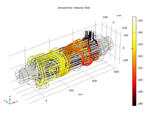
Locate the Coloring and Style section. Find the Line style subsection. From the Type list, choose Tube.
Color Expression 1
1
In the Velocity, Streamlines toolbar, click  Color Expression.
2
In the Settings window for Color Expression, click Replace Expression in the upper-right corner of the Expression section. From the menu, choose Component 1 (comp1)>Heat Transfer in Fluids>Temperature>T - Temperature - K.
3
Locate the Coloring and Style section. From the Color table list, choose Thermal.
Velocity, Streamlines
Evaluate the equivalent heat transfer coefficient by using the nonlocal couplings defined previously.
Heat Transfer Coefficient
1
In the Results toolbar, click  Global Evaluation.
2
In the Settings window for Global Evaluation, type Heat Transfer Coefficient in the Label text field.
3
Locate the Expressions section. In the table, enter the following settings:
The variable nitf1.qwf_u efficiently computes the heat flux through the wall separating water and air domains, based on the wall function definition.
4
Click  Evaluate.
To evaluate the pressure drop, the average inlet pressures are computed.
Inlet Pressure, Water
1
In the Results toolbar, click  More Derived Values and choose Average>Surface Average.
2
In the Settings window for Surface Average, type Inlet Pressure, Water in the Label text field.
3
Locate the Selection section. From the Selection list, choose Inlet Water.
4
Click Replace Expression in the upper-right corner of the Expressions section. From the menu, choose Component 1 (comp1)>Turbulent Flow, k-ε>Velocity and pressure>p - Pressure - Pa.
5
Click  Evaluate.
Inlet Pressure, Air
1
In the Results toolbar, click  More Derived Values and choose Average>Surface Average.
2
In the Settings window for Surface Average, type Inlet Pressure, Air in the Label text field.
3
Locate the Selection section. From the Selection list, choose Inlet Air.
4
Click Replace Expression in the upper-right corner of the Expressions section. From the menu, choose Component 1 (comp1)>Turbulent Flow, k-ε>Velocity and pressure>p - Pressure - Pa.
5
Click  Evaluate.
Table
1
Go to the Table window.
The tube side pressure drop is 36 Pa and the shell side pressure drop is 13 Pa.
Geometry Modeling Instructions
If you want to create the geometry yourself, follow these steps.
Geometry 1
1
In the Model Builder window, under Component 1 (comp1) click Geometry 1.
2
In the Settings window for Geometry, locate the Units section.
3
From the Length unit list, choose mm.
Cylinder 1 (cyl1)
1
In the Geometry toolbar, click  Cylinder.
2
In the Settings window for Cylinder, locate the Size and Shape section.
3
In the Radius text field, type 100.
4
In the Height text field, type 500.
5
Locate the Axis section. From the Axis type list, choose x-axis.
Cylinder 2 (cyl2)
1
In the Geometry toolbar, click  Cylinder.
2
In the Settings window for Cylinder, locate the Size and Shape section.
3
In the Radius text field, type 50.
4
In the Height text field, type 750.
5
Locate the Position section. In the x text field, type -125.
6
Locate the Axis section. From the Axis type list, choose x-axis.
Sphere 1 (sph1)
1
In the Geometry toolbar, click  Sphere.
2
In the Settings window for Sphere, locate the Size section.
3
In the Radius text field, type 100.
Sphere 2 (sph2)
1
In the Geometry toolbar, click  Sphere.
2
In the Settings window for Sphere, locate the Size section.
3
In the Radius text field, type 100.
4
Locate the Position section. In the x text field, type 500.
Cylinder 3 (cyl3)
1
In the Geometry toolbar, click  Cylinder.
2
In the Settings window for Cylinder, locate the Size and Shape section.
3
In the Radius text field, type 45.
4
In the Height text field, type 132.5.
5
Locate the Position section. In the x text field, type 50.
6
In the z text field, type -132.5.
Cylinder 4 (cyl4)
1
Right-click Cylinder 3 (cyl3) and choose Duplicate.
2
In the Settings window for Cylinder, locate the Position section.
3
In the x text field, type 450.
4
In the z text field, type 0.
Union 1 (uni1)
1
In the Geometry toolbar, click  Booleans and Partitions and choose Union.
2
Click in the Graphics window and then press Ctrl+A to select all objects.
3
In the Settings window for Union, locate the Union section.
4
Clear the Keep interior boundaries check box.
Block 1 (blk1)
1
In the Geometry toolbar, click  Block.
2
In the Settings window for Block, locate the Size and Shape section.
3
In the Width text field, type 500.
4
In the Depth text field, type 300.
5
In the Height text field, type 300.
6
Locate the Position section. In the y text field, type -150.
7
In the z text field, type -150.
8
Click to expand the Layers section. Find the Layer position subsection. Select the Right check box.
9
Clear the Bottom check box.
10
Block 2 (blk2)
1
In the Geometry toolbar, click  Block.
2
In the Settings window for Block, locate the Size and Shape section.
3
In the Width text field, type 500.
4
In the Depth text field, type 300.
5
In the Height text field, type 65.
6
Locate the Position section. In the y text field, type -150.
7
In the z text field, type -32.5.
Partition Objects 1 (par1)
1
In the Geometry toolbar, click  Booleans and Partitions and choose Partition Objects.
2
3
In the Settings window for Partition Objects, locate the Partition Objects section.
4
Find the Tool objects subsection. Select the  Activate Selection toggle button.
5
Select the objects blk1 and blk2 only.
Work Plane 1 (wp1)
1
In the Geometry toolbar, click  Work Plane.
2
In the Settings window for Work Plane, locate the Plane Definition section.
3
From the Plane list, choose yz-plane.
Work Plane 1 (wp1)>Plane Geometry
In the Model Builder window, click Plane Geometry.
Work Plane 1 (wp1)>Circle 1 (c1)
1
In the Work Plane toolbar, click  Circle.
2
In the Settings window for Circle, locate the Size and Shape section.
3
In the Radius text field, type 7.5.
4
Locate the Position section. In the xw text field, type -75.
5
In the yw text field, type -43.5.
Work Plane 1 (wp1)>Array 1 (arr1)
1
In the Work Plane toolbar, click  Transforms and choose Array.
2
3
In the Settings window for Array, locate the Size section.
4
In the xw size text field, type 7.
5
In the yw size text field, type 3.
6
Locate the Displacement section. In the xw text field, type 25.
7
In the yw text field, type 43.5.
Work Plane 1 (wp1)>Circle 2 (c2)
1
In the Model Builder window, under Component 1 (comp1)>Geometry 1>Work Plane 1 (wp1)>Plane Geometry right-click Circle 1 (c1) and choose Duplicate.
2
In the Settings window for Circle, locate the Position section.
3
In the xw text field, type -62.5.
4
In the yw text field, type -65.25.
Work Plane 1 (wp1)>Array 2 (arr2)
1
In the Work Plane toolbar, click  Transforms and choose Array.
2
3
In the Settings window for Array, locate the Size section.
4
In the xw size text field, type 6.
5
In the yw size text field, type 4.
6
Locate the Displacement section. In the xw text field, type 25.
7
In the yw text field, type 43.5.
8
Click  Build Selected.
Work Plane 1 (wp1)>Delete Entities 1 (del1)
1
In the Work Plane toolbar, click  Delete.
2
Select the objects arr1(1,1), arr1(1,3), arr1(7,1), arr1(7,3), arr2(1,1), arr2(1,4), arr2(6,1), and arr2(6,4) only.
Extrude 1 (ext1)
1
In the Model Builder window, under Component 1 (comp1)>Geometry 1 right-click Work Plane 1 (wp1) and choose Extrude.
2
In the Settings window for Extrude, locate the Distances section.
3
Block 3 (blk3)
1
In the Geometry toolbar, click  Block.
2
In the Settings window for Block, locate the Size and Shape section.
3
In the Width text field, type 1[m].
4
In the Depth text field, type 150.
5
In the Height text field, type 400.
6
Locate the Position section. In the x text field, type -200.
7
In the y text field, type -150.
8
In the z text field, type -200.
Difference 1 (dif1)
1
In the Geometry toolbar, click  Booleans and Partitions and choose Difference.
2
Select the objects ext1 and par1 only.
3
In the Settings window for Difference, locate the Difference section.
4
Find the Objects to subtract subsection. Select the  Activate Selection toggle button.
5
Ignore Faces 1 (igf1)
1
In the Geometry toolbar, click  Virtual Operations and choose Ignore Faces.
2
Click the  Go to Default View button in the Graphics toolbar.
3
Click the  Wireframe Rendering button in the Graphics toolbar.
4
On the object fin, select Boundaries 10, 17, 18, 25, 26, 32, 35, 38, 41, 52, 55, 58, 67, 70, 73, 76, 87, 90, 93, 102, 105, 112, 125, 132, 133, 138, 140, 141, 147, 150, 153, 156, 167, 170, 173, 182, 185, 188, 191, 202, 205, 208, 217, 220, 227, 234, 237, 244, 245, 252, 253, 259, 262, 265, 268, 279, 282, 285, 294, 297, 300, 303, 314, 317, 320, 329, 332, 339, 349, 356, 357, 362, 364, 365, 371, 374, 377, 380, 391, 394, 397, 406, 409, 412, 415, 426, 429, 432, 441, 444, 451, 458, 461, 468, 469, 476, 477, 483, 486, 489, 492, 503, 506, 509, 518, 521, 524, 527, 538, 541, 544, 553, 556, 563, 576, 578, 580, 582–587, and 589–598 only.
Water Domain
1
In the Geometry toolbar, click  Selections and choose Explicit Selection.
2
In the Settings window for Explicit Selection, type Water Domain in the Label text field.
3
On the object igf1, select Domain 1 only.
Air Domain
1
In the Geometry toolbar, click  Selections and choose Explicit Selection.
2
In the Settings window for Explicit Selection, type Air Domain in the Label text field.
3
On the object igf1, select Domain 2 only.
Water Domain, Exterior Boundaries
1
In the Geometry toolbar, click  Selections and choose Adjacent Selection.
2
In the Settings window for Adjacent Selection, type Water Domain, Exterior Boundaries in the Label text field.
3
Locate the Input Entities section. Click  Add.
4
In the Add dialog box, select Water Domain in the Input selections list.
5
Air Domain, Exterior Boundaries
1
In the Geometry toolbar, click  Selections and choose Adjacent Selection.
2
In the Settings window for Adjacent Selection, type Air Domain, Exterior Boundaries in the Label text field.
3
Locate the Input Entities section. Click  Add.
4
In the Add dialog box, select Air Domain in the Input selections list.
5
Baffles
1
In the Geometry toolbar, click  Selections and choose Adjacent Selection.
2
In the Settings window for Adjacent Selection, type Baffles in the Label text field.
3
Locate the Input Entities section. Click  Add.
4
In the Add dialog box, select Air Domain in the Input selections list.
5
6
In the Settings window for Adjacent Selection, locate the Output Entities section.
7
Select the Interior boundaries check box.
8
Clear the Exterior boundaries check box.
Symmetry
1
In the Geometry toolbar, click  Selections and choose Box Selection.
2
In the Settings window for Box Selection, type Symmetry in the Label text field.
3
Locate the Geometric Entity Level section. From the Level list, choose Boundary.
4
Locate the Box Limits section. In the y maximum text field, type 0.
5
Locate the Output Entities section. From the Include entity if list, choose Entity inside box.
Inlet Water
1
In the Geometry toolbar, click  Selections and choose Explicit Selection.
2
In the Settings window for Explicit Selection, type Inlet Water in the Label text field.
3
Locate the Entities to Select section. From the Geometric entity level list, choose Boundary.
4
On the object igf1, select Boundary 1 only.
Outlet Water
1
In the Geometry toolbar, click  Selections and choose Explicit Selection.
2
In the Settings window for Explicit Selection, type Outlet Water in the Label text field.
3
Locate the Entities to Select section. From the Geometric entity level list, choose Boundary.
4
On the object igf1, select Boundary 340 only.
Inlet Air
1
In the Geometry toolbar, click  Selections and choose Explicit Selection.
2
In the Settings window for Explicit Selection, type Inlet Air in the Label text field.
3
Locate the Entities to Select section. From the Geometric entity level list, choose Boundary.
4
On the object igf1, select Boundary 332 only.
Outlet Air
1
In the Geometry toolbar, click  Selections and choose Explicit Selection.
2
In the Settings window for Explicit Selection, type Outlet Air in the Label text field.
3
Locate the Entities to Select section. From the Geometric entity level list, choose Boundary.
4
On the object igf1, select Boundary 89 only.
Water Domain, Walls
1
In the Geometry toolbar, click  Selections and choose Difference Selection.
2
In the Settings window for Difference Selection, type Water Domain, Walls in the Label text field.
3
Locate the Geometric Entity Level section. From the Level list, choose Boundary.
4
Locate the Input Entities section. Click  Add.
5
In the Add dialog box, select Water Domain, Exterior Boundaries in the Selections to add list.
6
7
In the Settings window for Difference Selection, locate the Input Entities section.
8
9
In the Add dialog box, in the Selections to subtract list, choose Symmetry, Inlet Water, and Outlet Water.
10
Air Domain, Walls
1
In the Geometry toolbar, click  Selections and choose Difference Selection.
2
In the Settings window for Difference Selection, locate the Geometric Entity Level section.
3
From the Level list, choose Boundary.
4
In the Label text field, type Air Domain, Walls.
5
Locate the Input Entities section. Click  Add.
6
In the Add dialog box, in the Selections to add list, choose Air Domain, Exterior Boundaries and Baffles.
7
8
In the Settings window for Difference Selection, locate the Input Entities section.
9
10
In the Add dialog box, in the Selections to subtract list, choose Symmetry, Inlet Air, and Outlet Air.
11
Walls
1
In the Geometry toolbar, click  Selections and choose Union Selection.
2
In the Settings window for Union Selection, locate the Geometric Entity Level section.
3
From the Level list, choose Boundary.
4
Locate the Input Entities section. Click  Add.
5
In the Add dialog box, in the Selections to add list, choose Water Domain, Walls and Air Domain, Walls.
6
7
In the Settings window for Union Selection, type Walls in the Label text field.
Water-Air Interface
1
In the Geometry toolbar, click  Selections and choose Intersection Selection.
2
In the Settings window for Intersection Selection, type Water-Air Interface in the Label text field.
3
Locate the Geometric Entity Level section. From the Level list, choose Boundary.
4
Locate the Input Entities section. Click  Add.
5
In the Add dialog box, in the Selections to intersect list, choose Water Domain, Walls and Air Domain, Walls.
6
Interior Walls
1
In the Geometry toolbar, click  Selections and choose Union Selection.
2
In the Settings window for Union Selection, locate the Geometric Entity Level section.
3
From the Level list, choose Boundary.
4
Locate the Input Entities section. Click  Add.
5
In the Add dialog box, in the Selections to add list, choose Baffles and Water-Air Interface.
6
7
In the Settings window for Union Selection, type Interior Walls in the Label text field.