PDF

Sun’s Radiation Effect on Two Coolers Placed Under a Parasol
Introduction
A warm sunny day at the beach can be more enjoyable with a steady supply of frosty beverages. This example considers two Styrofoam coolers containing cold beverage cans sitting on a sandy beach. A parasol provides partial shade for one of the coolers over the course of the day. The difference in beverage temperature over time is computed. This tutorial demonstrates the usage of the external radiation source boundary condition, as well as how to model structures exposed to ambient conditions.
Figure 1: A parasol provides shade on the beach. Two Styrofoam coolers contain beverage cans that should remain as cold as possible.
Model Definition
A system of a parasol and two coolers is modeled as shown in Figure 1. The coolers, made of Styrofoam, contain six beverage cans each. The beverage cans are represented by water-filled cylinders with walls modeled as thermally thick thin layers of aluminum. The choice of the thermally thick option is not motivated by the physics, they are in reality thermally thin. With the thermally thick option a slit is defined for the temperature on the walls, so the temperature can differ between the inner and outer faces. This is used to define initial conditions that are discontinuous between the exterior and interior can surfaces. Because aluminum has higher thermal conductivity than the surrounding materials, the Thin Layer – thermally thick condition behaves like a continuity condition as soon as the initial temperature difference vanishes. The initial cans temperature is 1°C. The spacing between the cans and the cooler walls is small, so the model neglects free convection inside the cooler for simplicity.
The parasol primarily provides shade but otherwise has no significant thermal effect on the beverage temperature. For this reason, it is not too important to have a high fidelity model of the parasol. It is only the shadow cast by the parasol that contributes to the beverage temperature profile. The material used for the parasol is acrylic plastic.
The primary source of heat in this model is the solar irradiation, which is included using the External Radiation Source feature. This feature uses the longitude, latitude, time zone, time of year, and time of day to compute the direction of the incident solar radiation over the simulation time. Sun irradiance and temperature values recorded at Caracas, Venezuela (Meteorological data ASHRAE 2017) are chosen for this analysis. Assuming no cloud cover, the solar flux at the surface is about 1000 W/m2. All of the ambient surfaces of the model are included in the solar loading calculation, and shadowing effects are included.
The temperature of the sun is about 5800 K, and it emits primarily short-wavelength infrared and visible light at wavelengths shorter than 2.5 microns. The fraction of this short-wavelength solar radiation that is absorbed by the various materials is quantified by the solar absorptivity. Because the surfaces are at a much lower temperature, they reradiate in the long-wavelength infrared band, at wavelengths above 2.5 microns, and the fraction of reradiated energy is quantified by the surface emissivity. The solar and ambient wavelength dependence of emissivity model is used to account for differing emissivities in different wavelength bands.
There are three ambient temperature conditions in this model. First, the ground at 1 m below the sand surface is assumed to be at a constant temperature of 27°C throughout the day, corresponding to the average water temperature at this location.
The second ambient condition is the surrounding air temperature. There exists a combination of free and forced convection, due to wind, from all exposed surfaces to the ambient air, the temperature of which is assumed to vary sinusoidally through the day. In this application, the Convective Heat Flux boundary condition uses a bulk heat transfer coefficient of 20 W/(m2·K) for all exposed surfaces.
The third boundary condition is the radiative view factor to ambient. The graybody radiative view factors are computed between all exposed faces in the model, and radiative heat transfer is computed between these faces. However, these computed view factors do not sum to unity. There is a significant view factor to surrounding regions that is not modeled; this is the residual view factor. The temperature of the ambient is the same as the ambient air temperature.
Results and Discussion
Figure 2 plots the temperature profile at 4 p.m. Notice the decrease of temperature where the parasol shade stands.
Figure 2: Temperature distribution.
Figure 3 plots the temperature of the beverage inside two of the cans. This shows clearly the advantage of placing the cooler in the shade. At 2 p.m., the parasol shade starts to leave the cooler corresponding to the green curve, which is responsible for the sudden variation in the temperature increase at that moment.
Figure 3: Beverage temperature over time inside of the two coolers at the left side of the parasol (blue curve) and at the right side (green curve).
Reference
1. F.P. Incropera, D.P. DeWitt, T.L. Bergman, and A.S. Lavine, Fundamentals of Heat and Mass Transfer, 6th ed., John Wiley & Sons, 2006.
Application Library path: Heat_Transfer_Module/Thermal_Radiation/parasol
Modeling Instructions
From the File menu, choose New.
New
In the New window, click  Model Wizard.
Model Wizard
1
In the Model Wizard window, click  3D.
2
In the Select Physics tree, select Heat Transfer>Radiation>Heat Transfer with Surface-to-Surface Radiation.
3
Click Add.
4
Click  Study.
5
In the Select Study tree, select General Studies>Time Dependent.
6
Geometry 1
Define an analytic function for the time-dependent ambient temperature.
Global Definitions
Parameters 1
1
In the Model Builder window, under Global Definitions click Parameters 1.
2
In the Settings window for Parameters, locate the Parameters section.
3
Analytic 1 (an1)
1
In the Home toolbar, click  Functions and choose Global>Analytic.
2
In the Settings window for Analytic, type T_ambient in the Function name text field.
3
Locate the Definition section. In the Expression text field, type Tavg[1/K]+dT[1/K]*cos(2*pi*(x-14)/24).
4
Locate the Units section. In the Arguments text field, type h.
5
In the Function text field, type K.
6
Locate the Plot Parameters section. In the table, enter the following settings:
7
Geometry 1
Block 1 (blk1)
1
In the Geometry toolbar, click  Block.
2
In the Settings window for Block, locate the Size and Shape section.
3
In the Width text field, type 6.
4
In the Depth text field, type 6.
5
Locate the Position section. From the Base list, choose Center.
6
In the z text field, type -0.5.
7
Click  Build Selected.
This first block corresponds to a large region of sand. The next two blocks are the styrofoam coolers on the sand.
Block 2 (blk2)
1
In the Geometry toolbar, click  Block.
2
In the Settings window for Block, locate the Size and Shape section.
3
In the Width text field, type 0.3.
4
In the Depth text field, type 0.22.
5
In the Height text field, type 0.18.
6
Locate the Position section. From the Base list, choose Center.
7
In the x text field, type 0.5.
8
In the z text field, type 0.09.
9
Click  Build Selected.
Block 3 (blk3)
1
Right-click Block 2 (blk2) and choose Duplicate.
2
In the Settings window for Block, locate the Size and Shape section.
3
In the Width text field, type 0.26.
4
In the Depth text field, type 0.18.
5
In the Height text field, type 0.14.
6
Click  Build Selected.
In the next few steps, you create two six-pack cans by building one cylinder that is duplicated in two 3x2 arrays. Because the cans are located inside the two styrofoam coolers, you need to enable the Wireframe Rendering option to see them.
7
Click the  Wireframe Rendering button in the Graphics toolbar.
Cylinder 1 (cyl1)
1
In the Geometry toolbar, click  Cylinder.
2
In the Settings window for Cylinder, locate the Size and Shape section.
3
In the Radius text field, type 0.03.
4
In the Height text field, type 0.125.
5
Locate the Position section. In the x text field, type 0.42.
6
In the y text field, type 0.04.
7
In the z text field, type 0.02.
8
Click  Build Selected.
Array 1 (arr1)
1
In the Geometry toolbar, click  Transforms and choose Array.
2
3
In the Settings window for Array, locate the Size section.
4
In the x size text field, type 3.
5
In the y size text field, type 2.
6
Locate the Displacement section. In the x text field, type 0.08.
7
In the y text field, type -0.08.
8
Click  Build Selected.
Copy 1 (copy1)
1
In the Geometry toolbar, click  Transforms and choose Copy.
2
Select the objects arr1(1,1,1), arr1(1,2,1), arr1(2,1,1), arr1(2,2,1), arr1(3,1,1), arr1(3,2,1), blk2, and blk3 only.
For more convenience, use the Select Box button to select the abovementioned objects.
3
In the Settings window for Copy, locate the Displacement section.
4
In the x text field, type -1.5.
5
Click  Build Selected.
Now, create the parasol.
Cone 1 (cone1)
1
In the Geometry toolbar, click  Cone.
2
In the Settings window for Cone, locate the Size and Shape section.
3
In the Height text field, type 0.3.
4
From the Specify top size using list, choose Angle.
5
In the Semiangle text field, type 70.
6
Locate the Position section. In the z text field, type 1.5.
7
Click  Build Selected.
Cone 2 (cone2)
1
Right-click Cone 1 (cone1) and choose Duplicate.
2
In the Settings window for Cone, locate the Position section.
3
In the z text field, type 1.4.
4
Click  Build Selected.
Difference 1 (dif1)
1
In the Geometry toolbar, click  Booleans and Partitions and choose Difference.
2
3
In the Settings window for Difference, locate the Difference section.
4
Find the Objects to subtract subsection. Select the  Activate Selection toggle button.
5
6
Click  Build Selected.
Cylinder 2 (cyl2)
1
In the Geometry toolbar, click  Cylinder.
2
In the Settings window for Cylinder, locate the Size and Shape section.
3
In the Radius text field, type 0.05.
4
In the Height text field, type 1.7.
5
Click  Build Selected.
Form Union (fin)
1
In the Geometry toolbar, click  Build All.
2
Click the  Zoom Extents button in the Graphics toolbar.
Definitions
The following selection gathers the boundaries of the twelve cans.
Beverage Can Walls
1
In the Definitions toolbar, click  Explicit.
2
In the Settings window for Explicit, type Beverage Can Walls in the Label text field.
3
4
Locate the Output Entities section. From the Output entities list, choose Adjacent boundaries.
The next selection is for the irradiated surfaces.
Irradiated Surfaces
1
In the Definitions toolbar, click  Explicit.
2
In the Settings window for Explicit, type Irradiated Surfaces in the Label text field.
3
Locate the Input Entities section. From the Geometric entity level list, choose Boundary.
4
Add Material
1
In the Home toolbar, click  Add Material to open the Add Material window.
2
Go to the Add Material window.
3
In the tree, select Built-in>Water, liquid.
4
Click Add to Component in the window toolbar.
5
6
Click Add to Component in the window toolbar.
7
In the tree, select Built-in>Acrylic plastic.
8
Click Add to Component in the window toolbar.
9
In the tree, select Built-in>Aluminum.
10
Click Add to Component in the window toolbar.
Materials
Air (mat2)
1
In the Model Builder window, under Component 1 (comp1)>Materials click Air (mat2).
2
Acrylic plastic (mat3)
1
In the Model Builder window, click Acrylic plastic (mat3).
2
Can Walls
1
In the Model Builder window, under Component 1 (comp1)>Materials click Aluminum (mat4).
2
In the Settings window for Material, type Can Walls in the Label text field.
3
Locate the Geometric Entity Selection section. From the Geometric entity level list, choose Boundary.
4
From the Selection list, choose Beverage Can Walls.
Styrofoam
1
In the Materials toolbar, click  Blank Material.
2
In the Settings window for Material, type Styrofoam in the Label text field.
3
4
Locate the Material Contents section. In the table, enter the following settings:
Sand
1
In the Materials toolbar, click  Blank Material.
2
In the Settings window for Material, type Sand in the Label text field.
3
4
Locate the Material Contents section. In the table, enter the following settings:
5
In the Materials toolbar, click  Add Material to close the Add Material window.
Heat Transfer in Solids (ht)
Initial Values 1
1
In the Settings window for Initial Values, locate the Initial Values section.
2
In the T text field, type T_ambient(t).
Initial Values 2
1
In the Model Builder window, right-click Heat Transfer in Solids (ht) and choose Initial Values.
2
3
In the Settings window for Initial Values, locate the Initial Values section.
4
In the T text field, type 1[degC].
Temperature 1
1
In the Physics toolbar, click  Boundaries and choose Temperature.
2
3
In the Settings window for Temperature, locate the Temperature section.
4
In the T0 text field, type 27[degC].
Thin Layer 1
1
In the Physics toolbar, click  Boundaries and choose Thin Layer.
2
In the Settings window for Thin Layer, locate the Boundary Selection section.
3
From the Selection list, choose Beverage Can Walls.
Materials
Can Walls (mat4)
1
In the Model Builder window, under Component 1 (comp1)>Materials click Can Walls (mat4).
2
In the Settings window for Material, locate the Material Contents section.
3
Heat Transfer in Solids (ht)
Heat Flux 1
1
In the Physics toolbar, click  Boundaries and choose Heat Flux.
2
In the Settings window for Heat Flux, locate the Boundary Selection section.
3
From the Selection list, choose Irradiated Surfaces.
4
Locate the Heat Flux section. Click the Convective heat flux button.
5
In the h text field, type 20.
6
In the Text text field, type T_ambient(t).
Surface-to-Surface Radiation (rad)
1
In the Model Builder window, under Component 1 (comp1) click Surface-to-Surface Radiation (rad).
2
In the Settings window for Surface-to-Surface Radiation, locate the Boundary Selection section.
3
From the Selection list, choose Irradiated Surfaces.
4
Locate the Radiation Settings section. From the Wavelength dependence of radiative properties list, choose Solar and ambient.
Diffuse Surface 1
1
In the Model Builder window, under Component 1 (comp1)>Surface-to-Surface Radiation (rad) click Diffuse Surface 1.
2
In the Settings window for Diffuse Surface, locate the Ambient section.
3
Find the Ambient temperature subsection. In the Tamb text field, type T_ambient(t).
4
Locate the Surface Emissivity section. From the ε list, choose User defined for each band.
5
Diffuse Surface 2
1
In the Physics toolbar, click  Boundaries and choose Diffuse Surface.
2
3
In the Settings window for Diffuse Surface, locate the Ambient section.
4
Find the Ambient temperature subsection. In the Tamb text field, type T_ambient(t).
5
Locate the Surface Emissivity section. From the ε list, choose User defined for each band.
6
External Radiation Source 1
1
In the Physics toolbar, click  Global and choose External Radiation Source.
2
In the Settings window for External Radiation Source, locate the External Radiation Source section.
3
From the Source position list, choose Solar position.
4
From the Location defined by list, choose City.
5
From the list, choose Caracas, Venezuela.
6
In the Date table, enter the following settings:
7
In the Local time table, enter the following settings:
Study 1
Step 1: Time Dependent
1
In the Model Builder window, under Study 1 click Step 1: Time Dependent.
2
In the Settings window for Time Dependent, locate the Study Settings section.
3
From the Time unit list, choose h.
4
Click  Range.
5
In the Range dialog box, type 10 in the Start text field.
6
In the Step text field, type 10[min].
7
In the Stop text field, type 16.
8
Click Replace.
The study starts at 10 a.m. and ends at 4 p.m. with timesteps of 10 minutes.
9
In the Home toolbar, click  Compute.
Results
Surface 2
1
In the Model Builder window, expand the Temperature (ht) node, then click Surface 2.
2
In the Settings window for Surface, locate the Data section.
3
From the Solution parameters list, choose From parent.
4
Locate the Expression section. From the Unit list, choose degC.
Surface 1
1
In the Model Builder window, click Surface 1.
2
In the Settings window for Surface, locate the Expression section.
3
From the Unit list, choose degC.
4
Click the  Zoom Extents button in the Graphics toolbar.
The first default plot shows the temperature distribution as in Figure 2.
Isothermal Contours (ht)
The second default plot shows the isothermal contours.
Surface Radiosity (rad)
This default plot shows the surface radiosity. Proceed to plot the external irradiation at 2 p.m. and see the parasol shade as in Figure 1.
1
In the Model Builder window, click Surface Radiosity (rad).
2
In the Settings window for 3D Plot Group, locate the Data section.
3
From the Time (h) list, choose 12.
Radiosity
1
In the Model Builder window, expand the Surface Radiosity (rad) node, then click Radiosity.
2
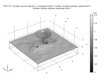
In the Settings window for Surface, click Replace Expression in the upper-right corner of the Expression section. From the menu, choose Component 1 (comp1)>Surface-to-Surface Radiation>Irradiation>Source heat flux - W/m²>rad.q0su1 - Source heat flux, 1 component.
3
Locate the Coloring and Style section. From the Color table list, choose GrayPrint.
4
In the Surface Radiosity (rad) toolbar, click  Plot.
Next, observe the temperature of the beverages as in Figure 3.
Temperature in the Coolers
1
In the Home toolbar, click  Add Plot Group and choose 1D Plot Group.
2
In the Settings window for 1D Plot Group, type Temperature in the Coolers in the Label text field.
Point Graph 1
1
In the Temperature in the Coolers toolbar, click  Point Graph.
2
For more convenience, you can click the Paste Selection button and paste the point numbers.
3
In the Settings window for Point Graph, locate the y-Axis Data section.
4
From the Unit list, choose degC.
5
In the Temperature in the Coolers toolbar, click  Plot.