PDF

Thermal Modeling of a Microchannel Heat Sink
Introduction
This example models a microchannel heat sink mounted on an active electronic component. The model geometry is based on the papers of Pak and others (Ref. 1) and by Jang and others (Ref. 2).
Thermal management has become a critical aspect of today’s electronic systems, which often include many high-performance circuits that dissipate large amounts of heat. Many of these components require efficient cooling to prevent overheating. Some of these components, such as processors, require a heat sink with cooling fins that are exposed to forced air from a fan. The microchannel heat sink featured in this tutorial has manifolds that work as flow dividers to improve its cooling performance (see Figure 1).
This tutorial analyze the temperature field in the air around the heat sink, inside the aluminum heat sink and the heat source. The governing energy transport is convection and conduction in the air domain, while the aluminum has pure conduction. A thermal contact resistance at the interface between the heat sink and the electronic component is also accounted for.
Figure 1: Microchannel heat sink with manifolds.
Model Definition
The model geometry consists of three domains: the electronic component, the aluminum heat sink, and the cooling air. Due to symmetry considerations, it is sufficient to model only a small element of the entire geometry as shown in Figure 2. Symmetry boundary conditions would then complete the model definition. In particular, the surfaces labeled Inlet and Outlet represent one quarter of the actual inlet and outlet.
This simulation uses the Conjugate Heat Transfer interface to solve for the coupled flow field in the air domain and the temperature field in the entire geometry.
Figure 2: Model geometry with symmetries.
Boundary conditions
A laminar inflow profile with an average velocity of 0.85 m/s at the inlet is used together with a prescribed temperature of 22°C. At the outlet the heat leaves through convection.
At the interface between the heat sink and electronic component, the Thermal Contact boundary condition is used. Thermal contact resistance is an important factor in the design of electronics cooling because it can significantly reduce a heat sink cooling performance. For more information about the thermal contact feature and its settings, read the theory section about the Thermal Contact feature in the Heat Transfer Module User’s Guide.
The surfaces of the heat sink and the ceramic heat source are not in perfect contact because of their roughness; air fills the gaps between the surfaces. Modeling the interface with the geometry of the rough surfaces would require a very dense mesh. An alternative, more practical, way of modeling the interface is to define a nonideal thermal contact, that is representative for the interface. In this case, the joint conductivity is the sum of the gap conductance hg and the conductivity due to the contact surface properties hc. The latter depends on the contact pressure, surface roughness and microhardness and is described by the Cooper-Mikic-Yovanovich correlation (Ref. 3).
Results and Discussion
Figure 3 shows the velocity profile via magnitude field and arrow plot in the air domain.
Figure 3: Velocity profile in the air domain.
Figure 4 shows the resulting temperature field in the heat sink with velocity streamlines in the air domain.
Figure 4: Temperature field and velocity streamlines in the heat sink.
At the ceramic-aluminum imperfect contact region, a small temperature jump appears due to light contact pressure. The average jump evaluates to 0.7 K and the joint conductance of the interface is about 8900 W/(m2·K).
References
1. B.C. Pak, W.C. Chun, B.J. Baek and D. Copeland, “Forced Air Cooling by Using Manifold Microchannel Heat Sinks”, Advances in Electronic Packaging, ASME-EEP, vol. 19, no. 2, pp. 1837–1842, 1997.
2. S.P. Jang, S.J. Kim and K.W. Paik, “Experimental Investigation of Thermal Characteristics for a Microchannel Heat Sink Subject to an Impinging Jet, Using a Micro-Thermal Sensor Array”, Sensors and Actuators A: Physical, vol. 105, no. 2, pp. 211–224, 2003.
3. M.M. Yovanovich and E.E. Marotta, “Thermal Spreading and Contact Resistance”, Heat Transfer Handbook, A. Bejan and A.D. Kraus eds., John Wiley & Sons, 2003.
Application Library path: Heat_Transfer_Module/Power_Electronics_and_Electronic_Cooling/microchannel_heat_sink
Modeling Instructions
From the File menu, choose New.
New
In the New window, click  Model Wizard.
Model Wizard
1
In the Model Wizard window, click  3D.
2
In the Select Physics tree, select Heat Transfer>Conjugate Heat Transfer>Laminar Flow.
3
Click Add.
4
Click  Study.
5
In the Select Study tree, select General Studies>Stationary.
6
Geometry 1
1
In the Model Builder window, under Component 1 (comp1) click Geometry 1.
2
In the Settings window for Geometry, locate the Units section.
3
From the Length unit list, choose mm.
Block 1 (blk1)
1
In the Geometry toolbar, click  Block.
2
In the Settings window for Block, locate the Size and Shape section.
3
In the Width text field, type 0.2.
4
In the Height text field, type 2.85.
5
Click to expand the Layers section. In the table, enter the following settings:
6
Click  Build Selected.
Block 2 (blk2)
1
In the Geometry toolbar, click  Block.
2
In the Settings window for Block, locate the Size and Shape section.
3
In the Width text field, type 0.1.
4
In the Height text field, type 1.4.
5
Locate the Position section. In the z text field, type 1.45.
6
Click  Build Selected.
Difference 1 (dif1)
1
In the Geometry toolbar, click  Booleans and Partitions and choose Difference.
2
3
In the Settings window for Difference, locate the Difference section.
4
Find the Objects to subtract subsection. Select the  Activate Selection toggle button.
5
6
Click  Build Selected.
Block 3 (blk3)
1
In the Geometry toolbar, click  Block.
2
In the Settings window for Block, locate the Size and Shape section.
3
In the Width text field, type 0.2.
4
In the Height text field, type 1.85.
5
Locate the Position section. In the z text field, type 1.45.
6
Click  Build Selected.
Difference 2 (dif2)
1
In the Geometry toolbar, click  Booleans and Partitions and choose Difference.
2
3
In the Settings window for Difference, locate the Difference section.
4
Find the Objects to subtract subsection. Select the  Activate Selection toggle button.
5
6
Select the Keep input objects check box.
7
Click  Build Selected.
Delete Entities 1 (del1)
1
In the Model Builder window, right-click Geometry 1 and choose Delete Entities.
2
In the Settings window for Delete Entities, locate the Entities or Objects to Delete section.
3
From the Geometric entity level list, choose Object.
4
5
Click  Build Selected.
Block 4 (blk4)
1
In the Geometry toolbar, click  Block.
2
In the Settings window for Block, locate the Size and Shape section.
3
In the Width text field, type 0.2.
4
In the Depth text field, type 0.5.
5
In the Height text field, type 0.45.
6
Locate the Position section. In the y text field, type 0.25.
7
In the z text field, type 2.85.
8
Click  Build Selected.
Difference 3 (dif3)
1
In the Geometry toolbar, click  Booleans and Partitions and choose Difference.
2
3
In the Settings window for Difference, locate the Difference section.
4
Find the Objects to subtract subsection. Select the  Activate Selection toggle button.
5
6
In the Geometry toolbar, click  Build All.
7
Click the  Zoom Extents button in the Graphics toolbar.
Define the parameters for the heat production and the contact pressure between the aluminum heat sink and the ceramic domain.
Global Definitions
Parameters 1
1
In the Model Builder window, under Global Definitions click Parameters 1.
2
In the Settings window for Parameters, locate the Parameters section.
3
Select the materials from the built-in material library.
Add Material
1
In the Home toolbar, click  Add Material to open the Add Material window.
2
Go to the Add Material window.
3
4
Click Add to Component in the window toolbar.
5
In the tree, select Built-in>Alumina.
6
Click Add to Component in the window toolbar.
7
In the tree, select Built-in>Aluminum 6063-T83.
8
Click Add to Component in the window toolbar.
9
In the Home toolbar, click  Add Material to close the Add Material window.
Materials
Alumina (mat2)
1
In the Model Builder window, under Component 1 (comp1)>Materials click Alumina (mat2).
2
Aluminum 6063-T83 (mat3)
1
In the Model Builder window, click Aluminum 6063-T83 (mat3).
2
Laminar Flow (spf)
1
In the Model Builder window, under Component 1 (comp1) click Laminar Flow (spf).
2
3
In the Settings window for Laminar Flow, locate the Domain Selection section.
4
Click  Create Selection.
5
In the Create Selection dialog box, type Air in the Selection name text field.
6
Inlet 1
1
In the Physics toolbar, click  Boundaries and choose Inlet.
2
3
In the Settings window for Inlet, locate the Boundary Condition section.
4
From the list, choose Fully developed flow.
5
Locate the Fully Developed Flow section. In the Uav text field, type 0.85.
Outlet 1
1
In the Physics toolbar, click  Boundaries and choose Outlet.
2
Symmetry 1
1
In the Physics toolbar, click  Boundaries and choose Symmetry.
2
Heat Transfer in Solids and Fluids (ht)
Fluid 1
1
In the Model Builder window, under Component 1 (comp1)>Heat Transfer in Solids and Fluids (ht) click Fluid 1.
2
In the Settings window for Fluid, locate the Domain Selection section.
3
From the Selection list, choose Air.
Heat Source 1
1
In the Physics toolbar, click  Domains and choose Heat Source.
2
3
In the Settings window for Heat Source, locate the Heat Source section.
4
In the Q0 text field, type Q_in.
Inflow 1
1
In the Physics toolbar, click  Boundaries and choose Inflow.
2
3
In the Settings window for Inflow, locate the Upstream Properties section.
4
In the Tustr text field, type 22[degC].
Outflow 1
1
In the Physics toolbar, click  Boundaries and choose Outflow.
2
Thermal Contact 1
1
In the Physics toolbar, click  Boundaries and choose Thermal Contact.
2
3
In the Settings window for Thermal Contact, locate the Thermal Contact section.
4
From the hg list, choose Parallel-plate gap gas conductance.
5
Locate the Contact Surface Properties section. In the σasp text field, type 1.5[um].
6
In the masp text field, type 0.2.
7
In the p text field, type P_c.
8
In the Hc text field, type 1[GPa].
9
Click to expand the Gap Properties section. From the kgap list, choose User defined.
Symmetry 1
1
In the Physics toolbar, click  Boundaries and choose Symmetry.
2
Mesh 1
The automatically generated mesh settings provide a good resolution for the fluid domains. In order to get a finer mesh in the solid domains, adjust the maximum element size for the solid domains.
Size
1
In the Model Builder window, under Component 1 (comp1) right-click Mesh 1 and choose Edit Physics-Induced Sequence.
2
In the Settings window for Size, click to expand the Element Size Parameters section.
3
In the Maximum element size text field, type 0.09.
4
Click  Build All.
5
In the Home toolbar, click  Compute.
Results
Velocity (spf)
The third default plot shows the velocity field in the air domain (see Figure 3).
1
In the Model Builder window, under Results click Velocity (spf).
Arrow Volume 1
1
In the Velocity (spf) toolbar, click  Arrow Volume.
2
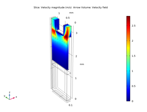
In the Settings window for Arrow Volume, click Replace Expression in the upper-right corner of the Expression section. From the menu, choose Component 1 (comp1)>Laminar Flow>Velocity and pressure>u,v,w - Velocity field.
3
Locate the Arrow Positioning section. Find the x grid points subsection. In the Points text field, type 5.
4
Find the z grid points subsection. In the Points text field, type 20.
5
Locate the Coloring and Style section. From the Color list, choose Black.
6
In the Velocity (spf) toolbar, click  Plot.
Evaluate the temperature jump and the joint conductance at the contact interface.
Temperature Jump and Joint Conductance
1
In the Results toolbar, click  More Derived Values and choose Average>Surface Average.
2
In the Settings window for Surface Average, type Temperature Jump and Joint Conductance in the Label text field.
3
4
Locate the Expressions section. In the table, enter the following settings:
The up and down operators return the temperature on each side of the contact boundary.
5
Click  Evaluate.
The temperature jump at the interface is about 0.45 K, and the joint conductance is about 13500 W/(m²·K).
To clearly distinguish the interface temperatures from the 3D temperature plot, follow the next steps.
Temperature (ht) 1
In the Model Builder window, right-click Temperature (ht) and choose Duplicate.
Surface 2
1
In the Model Builder window, expand the Temperature (ht) 1 node, then click Surface 2.
2
In the Settings window for Surface, click to expand the Inherit Style section.
3
From the Plot list, choose None.
Surface 1
In the Model Builder window, right-click Surface 1 and choose Delete.
Contact temperatures (ht)
1
In the Model Builder window, under Results click Temperature (ht) 1.
2
In the Settings window for 3D Plot Group, type Contact temperatures (ht) in the Label text field.
Upside
1
In the Model Builder window, under Results>Contact temperatures (ht) click Surface 2.
2
In the Settings window for Surface, type Upside in the Label text field.
3
Locate the Expression section. Select the Description check box.
4
5
Locate the Coloring and Style section. From the Color table list, choose ThermalLight.
Downside
1
In the Model Builder window, under Results>Contact temperatures (ht) click Surface 3.
2
In the Settings window for Surface, type Downside in the Label text field.
3
Locate the Expression section. Select the Description check box.
4
Deformation
1
In the Model Builder window, expand the Upside node, then click Deformation.
2
In the Settings window for Deformation, locate the Scale section.
3
In the Scale factor text field, type 2.
To reproduce the plot shown in Figure 4, follow the steps below.
Temperature (ht)
In the Model Builder window, expand the Results>Temperature (ht) node.
Surface 1, Surface 2, Surface 3
1
In the Model Builder window, under Results>Temperature (ht), Ctrl-click to select Surface 1, Surface 2, and Surface 3.
2
Temperature (ht)
In the Model Builder window, click Temperature (ht).
Slice 1
1
In the Temperature (ht) toolbar, click  Slice.
2
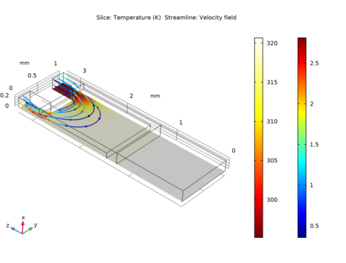
In the Settings window for Slice, click Replace Expression in the upper-right corner of the Expression section. From the menu, choose Component 1 (comp1)>Heat Transfer in Solids and Fluids>Temperature>T - Temperature - K.
3
Locate the Plane Data section. From the Entry method list, choose Coordinates.
4
Locate the Coloring and Style section. From the Color table list, choose ThermalLight.
Temperature (ht)
In the Model Builder window, click Temperature (ht).
Streamline 1
1
In the Temperature (ht) toolbar, click  Streamline.
2
In the Settings window for Streamline, click Replace Expression in the upper-right corner of the Expression section. From the menu, choose Component 1 (comp1)>Laminar Flow>Velocity and pressure>u,v,w - Velocity field.
3
4
Locate the Streamline Positioning section. In the Number text field, type 6.
5
Locate the Coloring and Style section. Find the Line style subsection. From the Type list, choose Tube.
6
Select the Radius scale factor check box.
7
In the Tube radius expression text field, type 0.006.
8
Find the Point style subsection. From the Type list, choose Arrow.
9
Select the Number of arrows check box.
10
Color Expression 1
1
In the Temperature (ht) toolbar, click  Color Expression.
2
In the Settings window for Color Expression, click Replace Expression in the upper-right corner of the Expression section. From the menu, choose Component 1 (comp1)>Laminar Flow>Velocity and pressure>spf.U - Velocity magnitude - m/s.
Definitions
In the Model Builder window, expand the Component 1 (comp1)>Definitions node.
Camera
1
In the Model Builder window, expand the Component 1 (comp1)>Definitions>View 1 node, then click Camera.
2
In the Settings window for Camera, locate the Camera section.
3
In the Zoom angle text field, type 7.
4
Locate the Position section. In the x text field, type 11.
5
In the y text field, type -11.
6
In the z text field, type -8.
7
Locate the Target section. In the x text field, type 0.1.
8
In the y text field, type 0.50.
9
In the z text field, type 1.66.
10
Locate the Up Vector section. In the x text field, type 0.8.
11
In the y text field, type 0.4.
12
In the z text field, type 0.4.
13
Locate the Center of Rotation section. In the z text field, type 1.66.
14
Locate the View Offset section. In the x text field, type 0.25.
15
In the y text field, type -0.25.
16
Click  Update.
Results
Temperature (ht)
1
In the Model Builder window, under Results click Temperature (ht).
2
In the Settings window for 3D Plot Group, locate the Plot Settings section.
3
From the View list, choose View 1.
4
In the Temperature (ht) toolbar, click  Plot.