PDF

LED Bulb Cooling
Introduction
This example simulates the thermodynamical behavior of a LED bulb, in order to evaluate the maximal temperature reached inside it while operating. It estimates the temperature of the system due to the heating of the LED chips, balanced by the cooling by a buoyancy driven air flow and radiation to the ambient surrounding.
In the past few years, light-emitting diode (LED) bulbs have progressively replaced incandescent light bulbs for both indoor and outdoor usage, due to their higher longevity and energy efficiency.
In LED bulbs, light emission is obtained by way of an electric current flowing through a semiconductor. In this physical process, called electroluminescence, 70% of the consumed electrical power is lost in heat. Therefore, to prevent from overheating, the geometry (size, number, and disposition of the LED chips, holes in the plastic bulb) and material properties (radiative properties of the aluminum PCB and plastic bulb) have to be optimized in the design of such devices.
In this model you compute the nonisothermal flow of air both inside and outside the bulb, by handling the coupling between energy transport — through conduction, radiation, and convection — and momentum transport induced by density variations of air.
Model Definition
The LED bulb considered in this study is made of acrylic plastic and has 6 holes at the top in order to let the air flow go through and remove heat.
It contains 8 lateral aluminum PCB supporting 18 LED chips each, and a top aluminum PCB supporting 12 LED chips. The total power of the bulb is 5 W. Radiation from the aluminum PCB to the ambient is handled in the computation. However, surface-to-surface radiation between the aluminum PCB and plastic bulb is neglected because most of the surfaces view factor is to the surrounding. Numerical simulations have shown that accounting for surface-to-surface radiation hardy changes the results while it increases significantly the computational cost.
The LED chips, made of epoxy resin, are welded on the aluminum PCB and dissipate each 70% of the electrical power they receive into heat, namely 3.5 W. The generated heat is transported to the surroundings through radiation, convection, and conduction. As air heats up, density and pressure changes induce a flow inside the bulb toward the top.
The base of the LED bulb is made of steel.
Flow regime
Before starting to implement the model into COMSOL Multiphysics, it is recommended to estimate the flow regime. The Rayleigh, Reynolds, Grashof, and Prandtl dimensionless numbers compare the viscous, buoyancy, thermal, and inertia effects and allow to qualify the flow as laminar or turbulent, and to decide for modeling settings.
These numbers are based on the order of magnitude of the main physical and geometric parameters of the system, summarized in Table 1 below.
1.8·10-5 Pa·s
n = μ/r
1.5·10-5 m2·s-1
3·10-3 K-1
2·10-5 m2·s-1
Grashof and Prandtl Numbers
The Grashof number compares the effect of buoyancy and viscous transportation, and is defined as
Thus, for this model, take gravity into account. Considering the parameters from Table 1, gives Gr = 107, which is below the critical number Grc = 109 over which the flow turns to be turbulent.
The Prandtl number indicates whether a stationary thermal regime is reachable or not by comparing the velocity of thermal effects with the one of the hydrodynamical effects:
The parameters from Table 1 give Pr = 0.5. This Prandtl number of order 1 indicates that the system will reach a thermal stationarity.
Rayleigh Number
The Rayleigh number Ra = Pr·Gr compares the buoyancy effects and the thermal diffusivity. It is needed to compute and estimate the typical velocity U of the fluid.
When the fluid is only led by buoyancy forces, its typical velocity U0 can be estimated from the Grashof number as
where ν/L is the speed due to viscous friction.
The velocity U, however, takes into account the thermal diffusivity. The Rayleigh number Ra = Pr(U0L/ν)2 also reads Ra = U2L/α with
U provides a more accurate velocity estimate as it takes the viscosity into account. The parameters in Table 1 give U = 0.28 m/s.
Reynolds Number
This number compares the effects of inertial forces to the viscous forces to which the fluid is submitted. It indicates whether the regime is laminar or turbulent, and is defined as
For a flow in a pipe, the threshold value from laminar to turbulent is about Re = 103. Using the parameters in Table 1 and the velocity estimate obtained from the Rayleigh number gives Re = 103, which corresponds to the transition threshold.
Flow Regime
All the dimensionless numbers computed above are summarized in Table 2 below.
Here the values of the Reynolds, the Grashof, and the estimated velocity justify to work under the hypothesis of a laminar flow. See Buoyancy Flow in Water tutorial for more details about the dimensionless numbers and their use.
Symmetry
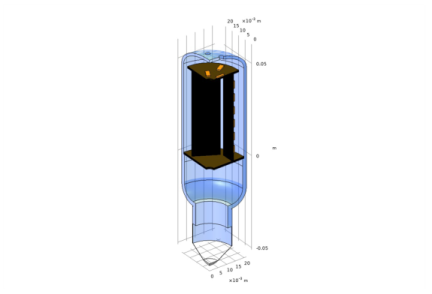
The LED geometry and the operating conditions have two obvious symmetry planes. As the flow regime is moderate, it is reasonable to assume that it shows the same symmetry. Hence it is possible to solve the equations on only the quarter of the geometry showed in Figure 1 and Figure 2, and to use symmetry conditions for the fluid flow and heat transfer equations. Numerical simulations using the full geometry have confirmed that the symmetry assumption for the flow does not modify the estimation of the cooling performance of the LED bulb.
Geometry
Figure 1 and Figure 2 show the LED bulb geometry used in the model. The LED chips and the aluminum PCB are represented in orange and brown, respectively.
Figure 1: A quarter of the LED bulb geometry. Front view, showing the LED chips position on the lateral PCB.
Figure 2: A quarter of the LED bulb geometry. View showing the LED chips position on the top PCP and the hole at the top of the bulb.
Real life system
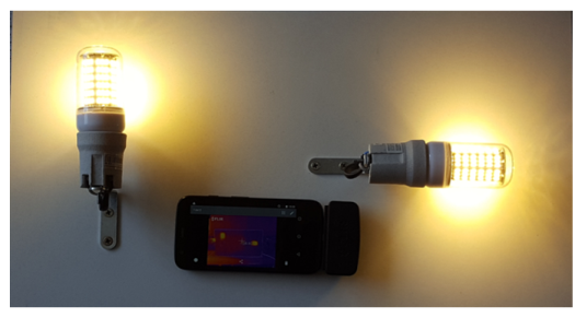
You can find LED bulbs similar to the one studied in this model in any hardware store. This section presents an experimental-like setup made up of two LED bulbs fixed on a vertical board (see Figure 3).
The LEDs are powered through a 230 V AC domestic current that is converted to an adapted current by the LED bulb electronic part that does not play any role in this thermodynamical study.
Figure 3: Device for experimental measurement.
The temperature is measured through a basic infrared camera (see Figure 4). Once the device reaches a stationary state, the maximal temperature observed through this disposal is around 72°C.
Figure 4: Temperature field given by an infrared camera.
Even if a more precise experiment would be needed in order to have a precise quantitative agreement between model and reality. This, nonetheless, acts like a proof of concept. In particular it confirmed, in agreement with the numerical results, that the cooling of the LED bulb is hardly influence by the orientation (vertical or horizontal).
Results and Discussion
The temperature distribution in the LED bulb is shown in Figure 5. A maximal temperature of about 76°C is obtained on the LED chips. This value is close to the experimental value displayed in Figure 4.
Figure 5: Temperature distribution with nominal power 5 W.
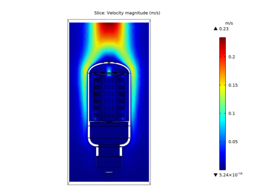
The velocity magnitude of the natural convection flow is shown in Figure 6. Its maximal value is about 0.2 m/s, which is close to the value estimated for U in the Flow regime section.
Figure 6: Velocity field magnitude.
Notes About the COMSOL Implementation
For this kind of buoyancy driven flow, a mainly vertical velocity is expected. Hence, in order to converge more easily toward the stationary solution, you can define a small positive value for vertical velocity initial condition. According to the calculation above, the initial velocity can be taken around 0.01 m/s.
Also due to the main direction of the flow, the normal dynamic pressure on the studied box of air the led bulb should not be ignored. The dynamic pressure is approximated to Pflow = ρrefw2/2, were w is the vertical velocity, and contributes to the total pressure, in addition the re reference and the static pressure that are already accounted for by default.
Application Library path: Heat_Transfer_Module/Power_Electronics_and_Electronic_Cooling/led_bulb
From the File menu, choose New.
New
In the New window, click  Model Wizard.
Model Wizard
1
In the Model Wizard window, click  3D.
2
In the Select Physics tree, select Heat Transfer>Conjugate Heat Transfer>Laminar Flow.
3
Click Add.
4
Click  Study.
5
In the Select Study tree, select General Studies>Stationary.
6
First, enter the parameters that will be needed to run the simulation.
Global Definitions
Parameters 1
1
In the Model Builder window, under Global Definitions click Parameters 1.
2
In the Settings window for Parameters, locate the Parameters section.
3
Geometry 1
Import 1 (imp1)
1
In the Home toolbar, click  Import.
2
In the Settings window for Import, locate the Import section.
3
Click Browse.
4
5
Click Import.
You should now see the geometry shown in Figure 1 and Figure 2. You can hide some parts to visualize the interior of the LED bulb.
6
Click the  Click and Hide button in the Graphics toolbar.
7
Click the  Select Boundaries button in the Graphics toolbar.
8
On the object imp1, select Boundary 44 only.
9
On the object imp1, select Boundary 261 only.
10
On the object imp1, select Boundary 43 only.
11
On the object imp1, select Boundary 41 only.
12
On the object imp1, select Boundary 42 only.
To simplify further selections, create some sets from now.
LED
1
In the Geometry toolbar, click  Selections and choose Explicit Selection.
2
In the Settings window for Explicit Selection, type LED in the Label text field.
3
On the object imp1, select Domains 8–28 and 30–41 only.
PCB
1
In the Geometry toolbar, click  Selections and choose Explicit Selection.
2
In the Settings window for Explicit Selection, type PCB in the Label text field.
3
On the object imp1, select Domains 4, 7, and 29 only.
4
Click the  Click and Hide button in the Graphics toolbar.
5
On the object imp1, select Domain 1 only.
6
On the object imp1, select Domain 3 only.
7
Click the  Click and Hide button in the Graphics toolbar.
8
On the object imp1, select Domains 4, 5, 7, and 29 only.
PCB Radiating Boundaries
1
In the Geometry toolbar, click  Selections and choose Explicit Selection.
2
In the Settings window for Explicit Selection, type PCB Radiating Boundaries in the Label text field.
3
Locate the Entities to Select section. From the Geometric entity level list, choose Boundary.
4
On the object imp1, select Boundaries 21, 49, 53, 82–87, 98, 126–131, 143, 169–174, 188, 189, and 249–260 only.
Outlet
1
In the Geometry toolbar, click  Selections and choose Explicit Selection.
2
In the Settings window for Explicit Selection, type Outlet in the Label text field.
3
Locate the Entities to Select section. From the Geometric entity level list, choose Boundary.
4
On the object imp1, select Boundary 13 only.
Inlet
1
In the Geometry toolbar, click  Selections and choose Explicit Selection.
2
In the Settings window for Explicit Selection, type Inlet in the Label text field.
3
Locate the Entities to Select section. From the Geometric entity level list, choose Boundary.
4
On the object imp1, select Boundaries 3, 44, and 261 only.
5
In the Geometry toolbar, click  Build All.
Before adding the materials, define which part of the system is solid and which one is fluid, in order to clarify the physics context.
Heat Transfer in Solids and Fluids (ht)
Fluid 1
1
In the Model Builder window, under Component 1 (comp1)>Heat Transfer in Solids and Fluids (ht) click Fluid 1.
2
In the Settings window for Fluid, locate the Domain Selection section.
3
Click  Paste Selection.
4
In the Paste Selection dialog box, type imp1: 1 in the Selection text field.
5
Laminar Flow (spf)
1
In the Model Builder window, under Component 1 (comp1) click Laminar Flow (spf).
2
In the Settings window for Laminar Flow, locate the Domain Selection section.
3
From the Selection list, choose Manual.
4
In the list, choose 2, 3 (hidden), 4, 5, 6, 7, 8, 9, 10, 11, 12, 13, 14, 15, 16, 17, 18, 19, 20, 21, 22, 23, 24, 25, 26, 27, 28, 29, 30, 31, 32, 33, 34, 35, 36, 37, 38, 39, 40, and 41.
5
Click  Remove from Selection.
6
Add Material
1
In the Home toolbar, click  Add Material to open the Add Material window.
2
Go to the Add Material window.
3
In the tree, select Built-in>Steel AISI 4340.
4
Click Add to Component in the window toolbar.
5
6
Click Add to Component in the window toolbar.
7
In the tree, select Built-in>Aluminum.
8
Click Add to Component in the window toolbar.
9
In the tree, select Built-in>Acrylic plastic.
10
Click Add to Component in the window toolbar.
11
In the tree, select Material Library>Epoxies>Filled epoxy resin (X238)>Filled epoxy resin (X238) [solid].
12
Click Add to Component in the window toolbar.
13
In the Home toolbar, click  Add Material to close the Add Material window.
Materials
Bulb base
1
In the Model Builder window, under Component 1 (comp1)>Materials click Steel AISI 4340 (mat1).
2
In the Settings window for Material, type Bulb base in the Label text field.
Air (mat2)
1
Click the  Transparency button in the Graphics toolbar.
2
Click the  View All button in the Graphics toolbar.
3
In the Model Builder window, click Air (mat2).
4
PCB
1
In the Model Builder window, under Component 1 (comp1)>Materials click Aluminum (mat3).
2
In the Settings window for Material, type PCB in the Label text field.
3
Locate the Geometric Entity Selection section. From the Selection list, choose PCB.
Plastic bulb
1
In the Model Builder window, under Component 1 (comp1)>Materials click Acrylic plastic (mat4).
2
In the Settings window for Material, type Plastic bulb in the Label text field.
3
LED chips
1
In the Model Builder window, under Component 1 (comp1)>Materials click Filled epoxy resin (X238) [solid] (mat5).
2
In the Settings window for Material, type LED chips in the Label text field.
3
Locate the Geometric Entity Selection section. From the Selection list, choose LED.
Add the heat capacity at constant pressure to the list of properties of the epoxy resin material.
4
Locate the Material Contents section. In the table, enter the following settings:
Laminar Flow (spf)
1
In the Model Builder window, under Component 1 (comp1) click Laminar Flow (spf).
2
Since the density variation is not small, the flow cannot be regarded as incompressible. Therefore set the flow to be compressible.
3
In the Settings window for Laminar Flow, locate the Physical Model section.
4
Select the Include gravity check box.
As the flow is driven by buoyancy, gravity matters.
5
Select the Use reduced pressure check box.
Initial Values 1
1
In the Model Builder window, under Component 1 (comp1)>Laminar Flow (spf) click Initial Values 1.
2
In the Settings window for Initial Values, locate the Initial Values section.
3
Specify the u vector as
Open Boundary 1
1
In the Physics toolbar, click  Boundaries and choose Open Boundary.
2
3
In the Settings window for Open Boundary, locate the Boundary Condition section.
4
In the f0 text field, type -0.5*spf.rhoref*w^2.
Open Boundary 2
1
In the Physics toolbar, click  Boundaries and choose Open Boundary.
2
Symmetry 1
1
In the Physics toolbar, click  Boundaries and choose Symmetry.
2
Heat Transfer in Solids and Fluids (ht)
In the Model Builder window, under Component 1 (comp1) click Heat Transfer in Solids and Fluids (ht).
Heat Source 1
1
In the Physics toolbar, click  Domains and choose Heat Source.
2
In the Settings window for Heat Source, locate the Domain Selection section.
3
From the Selection list, choose LED.
4
Locate the Heat Source section. Click the Heat rate button.
5
In the P0 text field, type heat_losses.
Surface-to-Ambient Radiation 1
1
In the Physics toolbar, click  Boundaries and choose Surface-to-Ambient Radiation.
2
In the Settings window for Surface-to-Ambient Radiation, locate the Boundary Selection section.
3
From the Selection list, choose PCB Radiating Boundaries.
4
5
Locate the Surface-to-Ambient Radiation section. From the ε list, choose User defined. In the associated text field, type 0.9.
Open Boundary 1
1
In the Physics toolbar, click  Boundaries and choose Open Boundary.
2
Symmetry 1
1
In the Physics toolbar, click  Boundaries and choose Symmetry.
2
Define the mesh manually to have enough cells within the thin parts of the geometry and precise boundary layers, without having to many elements.
Mesh 1
1
In the Model Builder window, under Component 1 (comp1) click Mesh 1.
2
In the Settings window for Mesh, locate the Mesh Settings section.
3
From the Sequence type list, choose User-controlled mesh.
Size
1
In the Model Builder window, under Component 1 (comp1)>Mesh 1 click Size.
2
In the Settings window for Size, locate the Element Size section.
3
Click the Custom button.
4
Click the Predefined button.
5
From the Predefined list, choose Coarse.
6
Click the Custom button.
7
Locate the Element Size Parameters section. In the Minimum element size text field, type 4e-4.
Size 1
1
In the Model Builder window, click Size 1.
2
In the Settings window for Size, locate the Element Size section.
3
From the Predefined list, choose Coarser.
Size 2
1
In the Model Builder window, click Size 2.
2
In the Settings window for Size, locate the Geometric Entity Selection section.
3
Click  Copy Selection.
4
Click  Zoom to Selection.
5
Click  Paste Selection.
6
In the Paste Selection dialog box, type 6 8 11 12 15 16 17 19 20 21 24 25 26 27 28 29 31 32 33 34 35 36 37 38 41 42 43 45 46 49 50 51 53 54 57 58 60 61 62 64 65 66 68 69 70 72 73 74 76 77 78 80 81 82 83 84 85 86 87 88 89 90 91 92 93 94 95 98 99 101 102 104 105 106 108 109 110 112 113 114 116 117 118 120 121 122 124 125 126 127 128 129 130 131 132 133 134 135 136 137 139 140 141 143 144 146 147 148 150 151 152 154 155 156 158 159 160 162 163 164 166 167 168 169 170 171 172 173 174 175 176 177 178 179 180 181 182 183 187 188 191 192 195 196 199 200 203 204 207 208 211 212 213 214 215 216 217 218 220 221 222 224 225 226 228 229 230 232 233 234 236 237 238 240 241 242 243 244 245 246 247 248 249 250 251 252 253 254 255 256 257 258 259 260 in the Selection text field.
7
8
In the Settings window for Size, locate the Geometric Entity Selection section.
9
10
Locate the Element Size section. Click the Custom button.
11
Click to collapse the Element Size Parameters section. Click to expand the Element Size Parameters section. Select the Minimum element size check box.
Boundary Layers 1
1
In the Model Builder window, click Boundary Layers 1.
2
In the Settings window for Boundary Layers, locate the Geometric Entity Selection section.
3
From the Selection list, choose All domains.
4
5
Click  Remove from Selection.
6
7
Click to expand the Corner Settings section.
Boundary Layer Properties 1
1
In the Model Builder window, expand the Boundary Layers 1 node, then click Boundary Layer Properties 1.
2
In the Settings window for Boundary Layer Properties, locate the Boundary Selection section.
3
Click  Paste Selection.
4
In the Paste Selection dialog box, type 6, 8, 11, 12, 15-17, 19-21, 24-29, 31-38, 41-43, 45, 46, 49-51, 53, 54, 57, 58, 60-62, 64-66, 68-70, 72-74, 76-78, 80-95, 98, 99, 101, 102, 104-106, 108-110, 112-114, 116-118, 120-122, 124-137, 139-141, 143, 144, 146-148, 150-152, 154-156, 158-160, 162-164, 166-183, 187, 188, 191, 192, 195, 196, 199, 200, 203, 204, 207, 208, 211-218, 220-222, 224-226, 228-230, 232-234, 236-238, 240-260 in the Selection text field.
5
6
In the Settings window for Boundary Layer Properties, click  Build All.
7
In the Home toolbar, click  Compute.
Results
Temperature (ht)
The Figure 6 and Figure 5 plots can be generated after the total geometry is recovered using a Mirror 3D. Follow the next steps to get to those plots.
Mirror 3D 1
1
In the Model Builder window, expand the Results>Datasets node.
2
Right-click Datasets and choose More 3D Datasets>Mirror 3D.
3
In the Settings window for Mirror 3D, click  Plot.
4
Click to expand the Advanced section. Select the Remove elements on the symmetry plane check box.
5
Mirror 3D 2
1
In the Results toolbar, click  More Datasets and choose Mirror 3D.
2
In the Settings window for Mirror 3D, locate the Data section.
3
From the Dataset list, choose Mirror 3D 1.
4
Locate the Plane Data section. From the Plane list, choose zx-planes.
5
Locate the Advanced section. Select the Remove elements on the symmetry plane check box.
6
Definitions
In the Model Builder window, expand the Component 1 (comp1)>Definitions node.
Hide for Geometry 1
1
In the Model Builder window, expand the Component 1 (comp1)>Definitions>View 1 node.
2
Right-click Hide for Geometry 1 and choose Disable.
Hide for Geometry 2
In the Model Builder window, right-click Hide for Geometry 2 and choose Disable.
Results
Mirror 3D 2
1
In the Model Builder window, under Results>Datasets click Mirror 3D 2.
2
In the Settings window for Mirror 3D, click  Plot.
Temperature (ht)
1
In the Model Builder window, click Temperature (ht).
2
In the Settings window for 3D Plot Group, locate the Data section.
3
From the Dataset list, choose Mirror 3D 2.
4
Locate the Color Legend section. Select the Show units check box.
5
Select the Show maximum and minimum values check box.
Surface
1
In the Model Builder window, expand the Temperature (ht) node, then click Surface.
2
In the Settings window for Surface, locate the Expression section.
3
From the Unit list, choose degC.
4
In the Temperature (ht) toolbar, click  Plot.
5
Click the  Transparency button in the Graphics toolbar.
6
Click the  Show Axis Orientation button in the Graphics toolbar.
7
Click the  Show Grid button in the Graphics toolbar.
Velocity (spf)
1
In the Model Builder window, expand the Results>Velocity (spf) node, then click Velocity (spf).
2
In the Settings window for 3D Plot Group, locate the Color Legend section.
3
Select the Show maximum and minimum values check box.
4
Select the Show units check box.
Slice
1
In the Model Builder window, click Slice.
2
In the Settings window for Slice, locate the Plane Data section.
3
In the Planes text field, type 1.
4
In the Velocity (spf) toolbar, click  Plot.
5
Click the  Go to YZ View button in the Graphics toolbar.
6
Locate the Data section. From the Dataset list, choose Mirror 3D 2.
7
In the Velocity (spf) toolbar, click  Plot.
8
Click the  Go to YZ View button in the Graphics toolbar.
9
Click the  Go to XZ View button in the Graphics toolbar.
10
Click the  Go to XY View button in the Graphics toolbar.
Velocity (spf)
1
In the Model Builder window, click Velocity (spf).
2
In the Settings window for 3D Plot Group, locate the Data section.
3
From the Dataset list, choose Mirror 3D 2.
4
In the Velocity (spf) toolbar, click  Plot.
5
Click the  Go to YZ View button in the Graphics toolbar.
6
Click the  Transparency button in the Graphics toolbar.