PDF

Heat Conduction in a Finite Slab
Introduction
This simple example covers the heat conduction in a finite slab, modeling how the temperature varies with time. You first set up the problem in COMSOL Multiphysics and then compare it to the analytical solution given in Ref. 1.
In addition, this example also shows how to avoid oscillations due to a jump between initial and boundary conditions by using a smoothed step function.
Model Definition
The model domain is defined between x = −b and x = b. The initial temperature is constant, equal to T0, over the whole domain; see the figure below. At time t = 0, the temperature at both boundaries is lowered to T1.
Figure 1: Modeling domain.
To compare the modeling results to the literature (Ref. 1), introduce new dimensionless variables according to the following definitions:
The model equation then becomes
with the associated initial condition
and boundary conditions
The analytical solution of this problem is (see Ref. 1, equation 12.1-31):
To model the temperature decrease at the boundaries use a smoothed step function of time f(τ).
This method is usually more realistic from a physical point of view than the sudden change in the temperature, and it is also better from a numerical point of view.
Results and Discussion
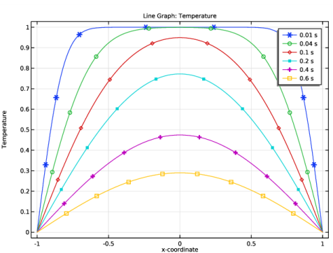
Figure 2 shows the temperature as a function of position at the dimensionless times τ = 0.01, 0.04, 0.1, 0.2, 0.4, and 0.6. In this plot, the slab’s center is situated at x = 0 with its end faces located a x = −1 and x = 1. The temperature profiles shown in the graph are identical to the analytical solution given in Ref. 1.
Figure 2: Temperature profiles.
The plot of the L2 error between the analytical and numerical solutions over time (see Figure 3) confirms this conclusion.
Figure 3: L2 error between analytical and numerical solutions over time.
Reference
1. R.B. Bird, W.E. Stewart, and E.N. Lightfoot, Transport Phenomena, 2nd ed., John Wiley & Sons, 2007.
Application Library path: Heat_Transfer_Module/Tutorials,_Conduction/heat_conduction_in_slab
Modeling Instructions
From the File menu, choose New.
New
In the New window, click  Model Wizard.
Model Wizard
1
In the Model Wizard window, click  1D.
2
In the Select Physics tree, select Heat Transfer>Heat Transfer in Solids (ht).
3
Click Add.
4
Click  Study.
5
In the Select Study tree, select General Studies>Time Dependent.
6
Geometry 1
The Heat Transfer in Solids interface can be used for solving the dimensionless equations. You can switch off the dimensions using the following commands:
Component 1 (comp1)
1
In the Model Builder window, click Component 1 (comp1).
2
In the Settings window for Component, locate the General section.
3
From the Unit system list, choose None.
Geometry 1
Interval 1 (i1)
1
In the Model Builder window, under Component 1 (comp1) right-click Geometry 1 and choose Interval.
2
In the Settings window for Interval, locate the Interval section.
3
4
Click  Build All Objects.
Definitions
Add a step function for use in the boundary conditions.
Step 1 (step1)
1
In the Home toolbar, click  Functions and choose Local>Step.
2
In the Settings window for Step, locate the Parameters section.
3
In the Location text field, type 1e-6.
4
In the From text field, type 1.
5
In the To text field, type 0.
6
Click to expand the Smoothing section. In the Size of transition zone text field, type 2e-6.
Optionally, you can inspect the shape of the step function.
7
Add a nonlocal integration coupling for the computation of the relative L2 error between numerical and analytical solutions.
Integration 1 (intop1)
1
In the Definitions toolbar, click  Nonlocal Couplings and choose Integration.
2
In the Settings window for Integration, locate the Source Selection section.
3
From the Selection list, choose All domains.
Heat Transfer in Solids (ht)
Solid 1
1
In the Model Builder window, under Component 1 (comp1)>Heat Transfer in Solids (ht) click Solid 1.
2
In the Settings window for Solid, locate the Heat Conduction, Solid section.
3
From the k list, choose User defined. In the associated text field, type 1.
4
Locate the Thermodynamics, Solid section. From the ρ list, choose User defined. In the associated text field, type 1.
5
From the Cp list, choose User defined. In the associated text field, type 1.
Initial Values 1
1
In the Model Builder window, click Initial Values 1.
2
In the Settings window for Initial Values, locate the Initial Values section.
3
In the T text field, type 1.
Temperature 1
1
In the Physics toolbar, click  Boundaries and choose Temperature.
2
Click in the Graphics window and then press Ctrl+A to select both boundaries.
3
In the Settings window for Temperature, locate the Temperature section.
4
In the T0 text field, type step1(t).
Mesh 1
1
In the Model Builder window, under Component 1 (comp1) click Mesh 1.
2
In the Settings window for Mesh, locate the Mesh Settings section.
3
From the Sequence type list, choose User-controlled mesh.
Size
1
In the Model Builder window, under Component 1 (comp1)>Mesh 1 click Size.
2
In the Settings window for Size, locate the Element Size section.
3
From the Predefined list, choose Finer.
Size 1
1
In the Model Builder window, right-click Edge 1 and choose Size.
2
In the Settings window for Size, locate the Geometric Entity Selection section.
3
From the Geometric entity level list, choose Boundary.
4
From the Selection list, choose All boundaries.
5
Locate the Element Size section. Click the Custom button.
6
Locate the Element Size Parameters section. Select the Maximum element size check box.
7
8
Click  Build All.
Study 1
Step 1: Time Dependent
1
In the Model Builder window, under Study 1 click Step 1: Time Dependent.
2
In the Settings window for Time Dependent, locate the Study Settings section.
3
In the Output times text field, type range(0,0.01,1).
To make sure that the transition of the boundary temperature from 1 to zero is represented correctly by the transient solver, use the initial time step that is smaller than the transition zone of the step function.
Solution 1 (sol1)
1
In the Study toolbar, click  Show Default Solver.
2
In the Model Builder window, expand the Solution 1 (sol1) node, then click Time-Dependent Solver 1.
3
In the Settings window for Time-Dependent Solver, click to expand the Time Stepping section.
4
Select the Initial step check box.
5
6
From the Maximum step constraint list, choose Constant.
7
In the Maximum step text field, type 1e-3.
8
In the Study toolbar, click  Compute.
Results
Temperature (ht)
The default plot shows the temperature distribution along the slab for all time steps. You can compare the computed solution to that of Ref. 1 by plotting the temperature for a given set of output times, as in Figure 2.
1
In the Settings window for 1D Plot Group, locate the Data section.
2
From the Time selection list, choose From list.
3
In the Times (s) list, choose 0.01, 0.04, 0.1, 0.2, 0.4, and 0.6.
4
In the Temperature (ht) toolbar, click  Plot.
Line Graph
1
In the Model Builder window, expand the Temperature (ht) node, then click Line Graph.
2
In the Settings window for Line Graph, click to expand the Legends section.
3
Select the Show legends check box.
4
Click to expand the Coloring and Style section. Find the Line markers subsection. From the Marker list, choose Cycle.
5
In the Temperature (ht) toolbar, click  Plot.
Next plot the relative L2 error between the numerical and analytical solutions over time.
Relative L2 Error
1
In the Home toolbar, click  Add Plot Group and choose 1D Plot Group.
2
In the Settings window for 1D Plot Group, type Relative L2 Error in the Label text field.
Line Graph 1
1
In the Relative L2 Error toolbar, click  Line Graph.
2
In the Settings window for Line Graph, locate the Selection section.
3
From the Selection list, choose All domains.
4
Locate the y-Axis Data section. In the Expression text field, type sqrt(intop1((T-2*sum((-1)^n/((n+0.5)*pi)*exp(-(n+0.5)^2*pi^2*t)*cos((n+0.5)*pi*x),n,0,1000))^2))/sqrt(intop1(T^2)).
5
Select the Description check box.
6
In the associated text field, type L2 error from analytical solution.
7
Locate the x-Axis Data section. From the Parameter list, choose Expression.
8
In the Expression text field, type t.
9
Locate the Coloring and Style section. From the Color list, choose Black.
10
In the Relative L2 Error toolbar, click  Plot.
As the analytical solution shows oscillations at initial time, change the settings of the graph for a better readability, to get the plot of Figure 3.
Relative L2 Error
1
In the Model Builder window, click Relative L2 Error.
2
In the Settings window for 1D Plot Group, locate the Axis section.
3
Select the Manual axis limits check box.
4
In the x minimum text field, type 1e-3.
5
In the x maximum text field, type 1.
6
In the y minimum text field, type 0.
7
In the y maximum text field, type 5e-4.
8
In the Relative L2 Error toolbar, click  Plot.