Viscous Heating in a Fluid Damper

Fluid dampers are used in military devices for shock isolation and in civil structures for suppressing earthquake-induced shaking and wind-induced vibrations, among many other applications. Fluid dampers work by dissipating the mechanical energy into heat (Ref. 1). This example shows the phenomenon of viscous heating and consequent temperature increase in a fluid damper. Viscous heating is also important in microflow devices, where a small cross-sectional area and large length of the device can generate significant heating and affect the fluid flow consequently (Ref. 2).

Model Definition

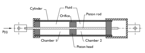
The structural elements of a fluid damper are relatively few. Figure 1 depicts a schematic of the fluid damper modeled herein with its main components: damper cylinder housing, piston rod, piston head, and viscous fluid in the chamber. There is a small annular space between the piston head and the inside wall of the cylinder housing. This acts as an effective channel for the fluid. As the piston head moves back and forth inside the damper cylinder, fluid is forced to pass through the annular channel with large shear rate, which leads to significant heat generation. The heat is transferred in both the axial and radial directions. In the radial direction, the heat is conducted through the cylinder house wall and convected to the air outside the damper, which is modeled using the Newton’s convective cooling law.

Figure 1: A sketch of a typical fluid damper with its major components.

You make use of the axially symmetric nature of the fluid damper and model it in a 2D-axisymmetric geometry as shown in Figure 2. The geometric dimensions and other parameters of the damper are taken according to Ref. 1 to represent the smaller, 15 kip damper experimentally studied therein. Thus, the piston head has a diameter of 8.37 cm, the piston rod diameter is 2.83 cm, and the gap thickness is about 1/100 of the piston head diameter. The damper has the maximum stroke U0 of 0.1524 m. The damper solid parts are made of steel, and the damping fluid is silicone oil.

Figure 2: Geometry and mesh. The domains (from left to right) represent: piston rod, piston head and damping fluid space, and the damper outer wall.

Fluid flow

The fluid flow in the fluid damper is described by the incompressible Navier-Stokes equations, solving for the velocity field u = (u, w) and the pressure p:

The density is assumed independent of the temperature, while the temperature dependence of the fluid viscosity is taken into account as:

(1)

The reference material properties of silicone oil are used.

No slip wall boundary conditions are applied for both ends of the damper cylinder and on the inner wall of the damper cylinder house. A Moving/sliding wall with the given velocity is applied on the boundaries of the piston head and on the piston rod.

Conjugate heat transfer

The conjugate heat transfer is solved both in the fluid domain and the damper cylinder house wall: heat transfer by convection and conduction in the fluid domain, heat transfer by conduction only in the solid domain, and the temperature field is continuous between the fluid and solid domains. In the fluid domain, the viscous dissipation is activated:

where the second term on the right-hand side represent the heat source from viscous dissipation. Hence, the problem is a fully coupled fluid-thermal interaction problem.

In the solid domain of the cylinder house wall, this equation reduces to conductive heat transfer equation without any heating source.

The heat flux boundary condition based on the Newton’s cooling law is applied on the outside boundaries of the cylinder house wall. The temperature field is continuous between the fluid and solid domains. The ends of the damper connected to the structures outside are kept at constant temperature.

The piston head movement is provided as harmonic oscillations with given amplitude and frequency, z = a0sin(2πf t), the piston head starting the simulation in its middle position. The motion is modeled using the arbitrary Lagrangian-Eulerian (ALE) deformed mesh. The ALE method handles the dynamics of the deforming geometry and the moving boundaries with a moving grid. The Navier-Stokes equations for fluid flow and heat equations for temperature variation are formulated in these moving coordinates.

Results and Discussion

The modeled loading has the amplitude of 0.127 m, and the excitation frequency is 0.4 Hz. This represents the long-stroke loading experiment performed in Ref. 1. The loading time period is 40 s.

Note that the simulation results for the temperature are presented in degrees Fahrenheit for the sake of easier comparison with the experimental measurements.

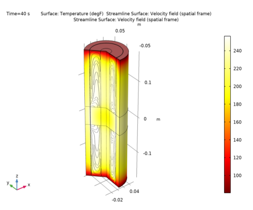
Figure 3 gives the temperature field in the damper at the end the loading. It also shows a typical streamline configuration for the flow induced in the damping fluid.

Figure 3: Temperature field in the damper at the end of simulation.

Figure 4 shows the temperature of the inner wall of the damper at the end-of-stroke position z = U0. This corresponds to the internal probe position under experiments performed in Ref. 1. The simulation results show very good agreement with the experimental measurements (see Fig. 9 in Ref. 1).

Figure 4: Temperature at the probe position.

Figure 5 shows the temperature variation along the inner wall of the damper after 10 s and 40 s of loading. It clearly shows that the temperature at the probe position does not represent the maximum temperature within the damper. This supports the conclusion drawn in Ref. 1, where the choice of the probe positioning was limited by the construction of the outer shell of the damper. Figure 5 also shows that the temperature near the center of the damper increases by about 100 degrees already after few loading cycles.

Figure 5: Temperature of the damper inner wall. The probe position corresponds to z ⁄ U0 = 1.

Notes About the COMSOL Implementation

You decompose the computational domain into several parts and mesh the domains with mapped meshes to resolve the very thin annular space. For the moving mesh you prescribe the displacement of the mesh in each domain so that their alignment remains unchanged with a zero displacement at the top and the bottom of the damper cylinder housing connecting to the high-performance seal, and the displacement equal to that of the piston head is used for the domain lined up with the piston head. This is achieved by specifying the mesh displacement field as a linear function of the deformed mesh frame coordinate and the reference (material) frame coordinate.

The steel material needed for the damper solid parts is available in the built-in material library. You create a user-defined material for the silicone oil. Such damping fluids are typically characterized by the density, kinematic viscosity at the temperature 25º C, and so-called viscosity temperature coefficient, VTC = 1−(viscosity at 98.9º C)/(viscosity at 37.8º C). Using this parameters, you create the linear correlation for the dynamic viscosity given by Equation 1.

References

1. C.J. Black and N. Makris, “Viscous Heating of Fluid Dampers Under Small and Large Amplitude Motions: Experimental Studies and Parametric Modeling”, J. Eng. Mech., vol. 133, pp. 566–577, 2007.

2. G.L. Morini, “Viscous Heating in Liquid Flows in Micro-Channels”, Int. J. Heat Mass Transfer, vol. 48, pp. 3637–3647, 2005.

Heat_Transfer_Module/Buildings_and_Constructions/fluid_damper

Modeling Instructions

From the menu, choose .

New

In the window, click

Model Wizard

In the window, click

In the tree, select .

Click .

Click

In the tree, select .

Click

Global Definitions

Parameters 1

In the window, under click .

In the window for , locate the section.

Click

Browse to the model’s Application Libraries folder and double-click the file fluid_damper_parameters.txt.

Piston displacement

In the toolbar, click

and choose .

In the window for , locate the section.

In the text field, type a0*sin(2*pi*f*t).

In the text field, type t.

Locate the section. In the text field, type s.

In the text field, type m.

Locate the section. In the table, enter the following settings:


Argument	Lower limit	Upper limit
t	0	40

Click

Click the

button in the toolbar.

In the text field, type zp.

Right-click and choose .

In the dialog box, type Piston displacement in the text field.

Click .

Definitions

Variables 1

In the toolbar, click

and choose .

In the window for , locate the section.

Click

Browse to the model’s Application Libraries folder and double-click the file fluid_damper_variables.txt.

Geometry 1

Rectangle 1 (r1)

In the toolbar, click

In the window for , locate the section.

In the text field, type Dr/2.

In the text field, type 2*Ld.

Locate the section. In the text field, type -Ld.

Rectangle 2 (r2)

In the toolbar, click

In the window for , locate the section.

In the text field, type Dp/2.

In the text field, type 2*Ld.

Locate the section. In the text field, type -Ld.

Rectangle 3 (r3)

In the toolbar, click

In the window for , locate the section.

In the text field, type Dd/2-Hw.

In the text field, type 2*Ld.

Locate the section. In the text field, type -Ld.

Rectangle 4 (r4)

In the toolbar, click

In the window for , locate the section.

In the text field, type Dd/2.

In the text field, type 2*Ld.

Locate the section. In the text field, type -Ld.

Rectangle 5 (r5)

In the toolbar, click

In the window for , locate the section.

In the text field, type Dd/2.

In the text field, type 2*Lp.

Locate the section. In the text field, type -Lp.

In the toolbar, click

Click the

button in the toolbar.

The model geometry is now complete.

Laminar Flow (spf)

In the window, under click .

Select Domains 4 and 6–9 only.

Heat Transfer in Solids and Fluids (ht)

Fluid 1

In the window, under click .

Select Domains 4 and 6–9 only.

In the window for , locate the section.

From the list, choose .

From the γ list, choose .

Add Material

In the toolbar, click

to open the window.

Go to the window.

In the tree, select .

Click in the window toolbar.

In the toolbar, click

to close the window.

Materials

In the following steps, you create a new material for the damping fluid, .

Silicone Oil

In the window, under right-click and choose .

In the window for , type Silicone Oil in the text field.

Select Domains 4 and 6–9 only.

In the window, expand the node, then click .

In the window for , locate the section.

Click

In the dialog box, type temperature in the text field.

Click

In the tree, select .

Click .

In the window for , locate the section.

In the table, enter the following settings:


Name	Expression	Unit	Description
nu_25C	0.0125[m^2/s]	m²/s
VTC	0.6[1]

In the window, under click .

In the window for , locate the section.

In the table, enter the following settings:


Property	Variable	Value	Unit	Property group
Thermal conductivity	k_iso ; kii = k_iso, kij = 0	22.5	W/(m·K)	Basic
Density	rho	950	kg/m³	Basic
Heat capacity at constant pressure	Cp	2e3	J/(kg·K)	Basic
Dynamic viscosity	mu	nu_25Crho(1-VTC(T-311[K])/(61[K]))/(1+VTC0.2107)	Pa·s	Basic