PDF

Evaporative Cooling of Water
Introduction
This tutorial shows how to simulate cooling of water including evaporative cooling. As an example, a beaker filled with water is used surrounded by an air domain. The airflow transports the water vapor which causes the liquid to cool down. The approach used here neglects volume change of the water inside the beaker. This is a reasonable assumption for problems where the considered time is short compared to the time needed to evaporate a noticeable amount of water.
Model Definition
The model geometry is shown in Figure 1. The size of the air domain is chosen such that increasing the domain would have no remarkable effect on the flow field around the beaker. Symmetry is used to reduce the model size.
Figure 1: Model geometry, using symmetry.
The beaker is made of glass and contains hot water at 80°C. The air has an initial temperature of 20°C and enters the modeling domain with this temperature.
For modeling evaporative cooling, three effects must be taken into account: turbulent flow of the air around the beaker, heat transfer in all domains, and transport of water vapor in the air. This is a real multiphysics problem and this tutorial shows how to set it up.
Turbulent Flow
The airflow is modeled with the Turbulent Flow, Low Re k-ε interface, because the Reynolds number is about 1500 and turbulent effects must be considered. In addition, they must be taken into account in the transport equations correctly. With the Low Re k-ε turbulence model, the turbulence variables are solved in the whole domain down to the walls and thus provide accurate input values for the transport equations. Using the assumption that the velocity and pressure field are independent of the air temperature and moisture content makes it possible to calculate the turbulent flow field in advance and then use it as input for the heat transfer and species transport equations.
Note that because the mass contribution due to the evaporation is small at the water surface, a wall (no slip) condition is used on this boundary for the airflow computation.
Heat Transfer
The heat transfer inside the beaker and water is due to conduction only. For the moist air, convection dominates the heat transfer and the turbulent flow field is required. The material properties are determined by the moist air theory.
During evaporation, latent heat is released from the water surface which cools down the water in addition to convective and conductive cooling by the surrounding. This additional heat flux depends on the amount of evaporated water. The latent heat source then is
(1)
The latent heat of vaporization Lvap is given in J/kg. The evaporative flux gevap is discussed in the next section.
Moisture Transport
To obtain the correct amount of water which is evaporated from the beaker into the air, the Moisture Transport in Air interface is used. The initial relative humidity is 20%. At the water surface evaporation occurs. The evaporative flux at the surface is
(2)
with the evaporation rate K, the molar mass of water vapor Mv, the vapor concentration cv and the saturation concentration csat which can be calculated from the correlation
(3)
The transport equation again uses the turbulent flow field as input. Turbulence must also be considered for the diffusion coefficient, by adding the following turbulent diffusivity to the diffusion tensor:
(4)
where νT is the turbulent kinematic viscosity, ScT is the turbulent Schmidt number, and I the unit matrix.
Results and Discussion
The image below shows the temperature field after 20 s with streamlines indicating the flow field.
Figure 2: Temperature distribution after 20 min and streamlines indicating the flow field.
Due to convection, conduction, and evaporation the water cools down over time. As shown in Figure 3 the average temperature after 20 min is about 31°C.
Figure 3: Average water temperature over time.
Figure 4 shows the concentration and relative humidity at the symmetry plane. Close to the water surface, the relative humidity is about 100% as expected. Behind the beaker the relative humidity can become even smaller than 20%. Due to the high temperature, air can absorb a higher amount of water.
Figure 4: Concentration distribution and contour lines for the relative humidity.
The last study computes for a situation where the evaporation effects are neglected. Figure 5 shows the comparison between average water temperatures with and without evaporation to see the its importance in the cooling process. A difference of approximately 10 K can be observed.
Figure 5: Average water temperature with and without evaporation accounted.
Application Library path: Heat_Transfer_Module/Phase_Change/evaporative_cooling
Modeling Instructions
The first step is to compute the turbulent flow field. After that, the resulting velocity field will be used to compute the transport of heat and moisture. To get an accurate velocity field for the turbulent transport equations, the Low-Reynolds k-ε turbulence model is used here.
From the File menu, choose New.
New
In the New window, click  Model Wizard.
Model Wizard
1
In the Model Wizard window, click  3D.
2
In the Select Physics tree, select Fluid Flow>Single-Phase Flow>Turbulent Flow>Turbulent Flow, Low Re k-ε (spf).
3
Click Add.
4
Click  Study.
5
In the Select Study tree, select Preset Studies for Selected Physics Interfaces>Stationary with Initialization.
6
Geometry 1
Load the geometry sequence from an existing MPH file.
1
In the Geometry toolbar, click  Insert Sequence.
2
3
In the Geometry toolbar, click  Build All.
4
Click the  Wireframe Rendering button in the Graphics toolbar.
5
Click the  Zoom Extents button in the Graphics toolbar.
The flow calculation is done for the air domain only. For now, air is the only material you need.
Add Material
1
In the Home toolbar, click  Add Material to open the Add Material window.
2
Go to the Add Material window.
3
4
Click Add to Component in the window toolbar.
5
In the Home toolbar, click  Add Material to close the Add Material window.
Turbulent Flow, Low Re k-ε (spf)
1
In the Model Builder window, under Component 1 (comp1) click Turbulent Flow, Low Re k-ε (spf).
2
In the Settings window for Turbulent Flow, Low Re k-ε, locate the Turbulence section.
3
From the Wall treatment list, choose Low Re.
This makes sure that the flow field is resolved down to the wall everywhere.
4
Locate the Domain Selection section. Click  Clear Selection.
5
Create a selection from this domain. It can be used later to create new selections or to assign physical properties.
6
Click  Create Selection.
7
In the Create Selection dialog box, type Air in the Selection name text field.
8
Now, define the boundary conditions.
Inlet 1
1
In the Physics toolbar, click  Boundaries and choose Inlet.
2
3
In the Settings window for Inlet, locate the Velocity section.
4
In the U0 text field, type 2.
Open Boundary 1
1
In the Physics toolbar, click  Boundaries and choose Open Boundary.
2
Symmetry 1
1
In the Physics toolbar, click  Boundaries and choose Symmetry.
2
Mesh 1
Customize the mesh, so that it resolves both, the fluid flow and later the transport of heat and moisture properly. Use the Physics-controlled mesh as starting point.
1
In the Model Builder window, under Component 1 (comp1) click Mesh 1.
2
In the Settings window for Mesh, locate the Physics-Controlled Mesh section.
3
From the Element size list, choose Extra coarse.
4
Locate the Mesh Settings section. From the Sequence type list, choose User-controlled mesh.
Size
1
In the Model Builder window, under Component 1 (comp1)>Mesh 1 click Size.
2
In the Settings window for Size, locate the Element Size section.
3
From the Predefined list, choose Coarse.
4
Click the Custom button.
5
Locate the Element Size Parameters section. In the Minimum element size text field, type 1.
Size 2
1
In the Model Builder window, click Size 2.
2
3
In the Settings window for Size, locate the Element Size section.
4
From the Predefined list, choose Coarse.
5
Click  Build Selected.
Size 3
1
Right-click Component 1 (comp1)>Mesh 1>Size 2 and choose Duplicate.
2
In the Settings window for Size, locate the Element Size section.
3
From the Predefined list, choose Fine.
4
Locate the Geometric Entity Selection section. Click  Clear Selection.
5
6
Locate the Element Size section. Click the Custom button.
7
Locate the Element Size Parameters section. Select the Maximum element size check box.
8
Strong gradients appear near the water surface for both velocity, temperature and moisture content. Make the mesh elements smaller close the surface to improve accuracy.
Free Tetrahedral 1
1
In the Model Builder window, click Free Tetrahedral 1.
2
In the Settings window for Free Tetrahedral, locate the Domain Selection section.
3
From the Selection list, choose All domains.
Boundary Layers 1
1
In the Model Builder window, click Boundary Layers 1.
2
In the Settings window for Boundary Layers, click to expand the Corner Settings section.
3
In the Minimum angle for trimming text field, type 350.
Boundary Layer Properties 1
1
In the Model Builder window, expand the Boundary Layers 1 node, then click Boundary Layer Properties 1.
2
In the Settings window for Boundary Layer Properties, locate the Boundary Layer Properties section.
3
In the Number of boundary layers text field, type 4.
4
In the Model Builder window, right-click Mesh 1 and choose Build All.
Study 1
In the Home toolbar, click  Compute.
Results
Velocity (spf)
1
Click the  Go to Default View button in the Graphics toolbar.
2
Click the  Zoom Extents button in the Graphics toolbar.
The resulting velocity field is shown below:
With this velocity field, the transport equations can be computed. The Heat Transfer in Moist Air together with the Moisture Transport in Air interface are used to describe the transport of heat and moist air and the interaction of both processes.
Add Physics
1
In the Home toolbar, click  Add Physics to open the Add Physics window.
2
Go to the Add Physics window.
3
In the tree, select Heat Transfer>Heat and Moisture Transport>Moist Air.
4
Find the Physics interfaces in study subsection. In the table, clear the Solve check box for Study 1.
5
Click Add to Component 1 in the window toolbar.
6
In the Home toolbar, click  Add Physics to close the Add Physics window.
Global Definitions
Parameters 1
1
In the Model Builder window, under Global Definitions click Parameters 1.
2
In the Settings window for Parameters, locate the Parameters section.
3
The evaporation rate is chosen so that the solution is not affected if the rate is further increased. This corresponds to assuming that vapor is in equilibrium with the liquid.
Materials
Add the materials for heat transfer calculations in the cup and water.
Add Material
1
In the Home toolbar, click  Add Material to open the Add Material window.
2
Go to the Add Material window.
3
In the tree, select Built-in>Water, liquid.
4
Click Add to Component in the window toolbar.
Materials
Water, liquid (mat2)
1
2
In the Settings window for Material, locate the Geometric Entity Selection section.
3
Click  Create Selection.
4
In the Create Selection dialog box, type Water in the Selection name text field.
5
With this selection and the one for the air domain, it is easy to create the selection for the glass body.
Definitions
Glass
1
In the Model Builder window, expand the Component 1 (comp1)>Definitions node.
2
Right-click Definitions and choose Selections>Complement.
3
In the Settings window for Complement, type Glass in the Label text field.
4
Locate the Input Entities section. Under Selections to invert, click  Add.
5
In the Add dialog box, in the Selections to invert list, choose Air and Water.
6
Add Material
1
Go to the Add Material window.
2
In the tree, select Built-in>Glass (quartz).
3
Click Add to Component in the window toolbar.
4
In the Home toolbar, click  Add Material to close the Add Material window.
Materials
Glass (quartz) (mat3)
1
In the Settings window for Material, locate the Geometric Entity Selection section.
2
From the Selection list, choose Glass.
Heat Transfer in Moist Air (ht)
Add a Fluid node for the water domain. To save computational time, the velocity field driven by natural convection is not computed. Instead, an increased thermal conductivity determined by built-in Nusselt number correlations is defined in the next steps to compensate the missing convective heat flux.
1
In the Model Builder window, under Component 1 (comp1) click Heat Transfer in Moist Air (ht).
Fluid 1
1
In the Physics toolbar, click  Domains and choose Fluid.
2
Convectively Enhanced Conductivity 1
1
In the Physics toolbar, click  Attributes and choose Convectively Enhanced Conductivity.
2
In the Settings window for Convectively Enhanced Conductivity, locate the Convectively Enhanced Conductivity section.
3
From the Nusselt number correlation list, choose Vertical rectangular cavity.
4
In the H text field, type 8[cm].
5
In the L text field, type 3.5[cm].
Then, add a Solid node for the glass domain.
Solid 1
1
In the Physics toolbar, click  Domains and choose Solid.
2
In the Settings window for Solid, locate the Domain Selection section.
3
From the Selection list, choose Glass.
The air enters the domain at room temperature. At the outlet, the heat is transported away by convection.
Inflow 1
1
In the Physics toolbar, click  Boundaries and choose Inflow.
2
Open Boundary 1
1
In the Physics toolbar, click  Boundaries and choose Open Boundary.
2
Symmetry 1
1
In the Physics toolbar, click  Boundaries and choose Symmetry.
2
Click the  Go to YZ View button in the Graphics toolbar.
With this tool, draw a box around all symmetry boundaries, which corresponds to:
3
You should see the following in your Graphics window:
The fluid in the beaker has an initial temperature of 80°C.
Initial Values 2
1
In the Physics toolbar, click  Domains and choose Initial Values.
2
3
In the Settings window for Initial Values, locate the Domain Selection section.
4
From the Selection list, choose Water.
5
Locate the Initial Values section. In the T text field, type 80[degC].
Set up the Moisture Transport in Air interface.
Moisture Transport in Air (mt)
1
In the Model Builder window, under Component 1 (comp1) click Moisture Transport in Air (mt).
2
In the Settings window for Moisture Transport in Air, locate the Domain Selection section.
3
From the Selection list, choose Air.
Initial Values 1
1
In the Model Builder window, under Component 1 (comp1)>Moisture Transport in Air (mt) click Initial Values 1.
2
In the Settings window for Initial Values, locate the Initial Values section.
3
In the φw,0 text field, type phi0.
Inflow 1
1
In the Physics toolbar, click  Boundaries and choose Inflow.
2
3
In the Settings window for Inflow, locate the Upstream Properties section.
4
In the φw,ustr text field, type phi0.
Open Boundary 1
1
In the Physics toolbar, click  Boundaries and choose Open Boundary.
2
3
In the Settings window for Open Boundary, locate the Upstream Properties section.
4
In the φw,ustr text field, type phi0.
Symmetry 1
1
In the Physics toolbar, click  Boundaries and choose Symmetry.
2
Wet Surface 1
1
In the Physics toolbar, click  Boundaries and choose Wet Surface.
2
3
In the Settings window for Wet Surface, locate the Wet Surface Settings section.
4
In the K text field, type K.
Now, set up the multiphysics couplings for moisture and heat transport by the airflow. Start with a fictive model where latent heat source due to evaporation is neglected.
Multiphysics
Heat and Moisture 1 (ham1)
1
In the Model Builder window, under Component 1 (comp1)>Multiphysics click Heat and Moisture 1 (ham1).
2
In the Settings window for Heat and Moisture, locate the Latent Heat section.
3
Clear the Include latent heat source on surfaces check box.
Nonisothermal Flow 1 (nitf1)
1
In the Physics toolbar, click  Multiphysics Couplings and choose Domain>Nonisothermal Flow.
2
In the Settings window for Nonisothermal Flow, locate the Material Properties section.
3
Select the Boussinesq approximation check box.
Couple the flow and pressure field.
Moisture Flow 1 (mf1)
1
In the Physics toolbar, click  Multiphysics Couplings and choose Domain>Moisture Flow.
To keep Study 1 in its original state, deselect these last two multiphysics coupling features from the study tables.
Study 1
Step 1: Wall Distance Initialization
1
In the Model Builder window, under Study 1 click Step 1: Wall Distance Initialization.
2
In the Settings window for Wall Distance Initialization, locate the Physics and Variables Selection section.
3
In the table, clear the Solve for check boxes for Nonisothermal Flow 1 (nitf1) and Moisture Flow 1 (mf1).
Step 2: Stationary
1
In the Model Builder window, click Step 2: Stationary.
2
In the Settings window for Stationary, locate the Physics and Variables Selection section.
3
In the table, clear the Solve for check boxes for Nonisothermal Flow 1 (nitf1) and Moisture Flow 1 (mf1).
Add Study
1
In the Home toolbar, click  Add Study to open the Add Study window.
2
Go to the Add Study window.
3
Find the Physics interfaces in study subsection. In the table, clear the Solve check box for Turbulent Flow, Low Re k-ε (spf).
4
Find the Studies subsection. In the Select Study tree, select General Studies>Time Dependent.
5
Click Add Study in the window toolbar.
6
In the Home toolbar, click  Add Study to close the Add Study window.
Study 2 : no latent heat source
1
In the Model Builder window, click Study 2.
2
In the Settings window for Study, type Study 2 : no latent heat source in the Label text field.
Step 1: Time Dependent
Due to the Wet Surface boundary condition, the time-dependent simulation of heat- and moisture transport is very sensitive to the choice of the time dependent solver settings. Tune the solver, by restricting the time step size.
1
In the Model Builder window, under Study 2 : no latent heat source click Step 1: Time Dependent.
2
In the Settings window for Time Dependent, locate the Study Settings section.
3
From the Time unit list, choose min.
4
In the Output times text field, type range(0,20[s],20).
5
Click to expand the Values of Dependent Variables section. Find the Values of variables not solved for subsection. From the Settings list, choose User controlled.
6
From the Method list, choose Solution.
7
From the Study list, choose Study 1, Stationary.
Because you do not solve for the flow field again, but want to use the results from the first study, you have to tell the time-dependent study that the results from the stationary study should be used.
Solution 3 (sol3)
1
In the Study toolbar, click  Show Default Solver.
2
In the Model Builder window, expand the Solution 3 (sol3) node, then click Time-Dependent Solver 1.
3
In the Settings window for Time-Dependent Solver, click to expand the Time Stepping section.
4
From the Maximum step constraint list, choose Constant.
5
In the Maximum step text field, type 1.
6
Right-click Time-Dependent Solver 1 and choose Fully Coupled.
7
In the Settings window for Fully Coupled, click to expand the Method and Termination section.
8
From the Jacobian update list, choose On every iteration.
Step 1: Time Dependent
In the Study toolbar, click  Compute.
Results
Temperature (ht)
Create the plot shown in Figure 2.
Surface 2
1
In the Results toolbar, click  More Datasets and choose Surface.
2
In the Settings window for Surface, locate the Data section.
3
From the Dataset list, choose Study 2 : no latent heat source/Solution 3 (sol3).
4
Locate the Selection section. From the Selection list, choose All boundaries.
5
Temperature (ht)
1
In the Model Builder window, click Temperature (ht).
2
In the Settings window for 3D Plot Group, locate the Data section.
3
From the Dataset list, choose Surface 2.
Surface
1
In the Model Builder window, expand the Temperature (ht) node, then click Surface.
2
In the Settings window for Surface, locate the Expression section.
3
From the Unit list, choose degC.
Temperature (ht)
In the Model Builder window, click Temperature (ht).
Streamline 1
1
In the Temperature (ht) toolbar, click  Streamline.
2
In the Settings window for Streamline, locate the Data section.
3
From the Dataset list, choose Study 2 : no latent heat source/Solution 3 (sol3).
4
From the Solution parameters list, choose From parent.
5
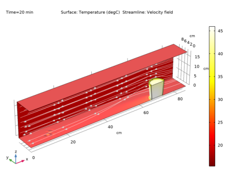
Locate the Coloring and Style section. Find the Point style subsection. From the Color list, choose White.
6
Locate the Streamline Positioning section. From the Positioning list, choose On selected boundaries.
7
Locate the Selection section. Select the  Activate Selection toggle button.
8
9
Locate the Coloring and Style section. From the Type list, choose Arrow.
10
Select the Number of arrows check box.
11
12
In the Temperature (ht) toolbar, click  Plot.
13
Click the  Go to Default View button in the Graphics toolbar.
To visualize the moisture distribution as in Figure 4, follow the next steps.
Cut Plane 1
1
In the Results toolbar, click  Cut Plane.
2
In the Settings window for Cut Plane, locate the Plane Data section.
3
From the Plane list, choose xz-planes.
4
Locate the Data section. From the Dataset list, choose Study 2 : no latent heat source/Solution 3 (sol3).
Moisture Concentration and Relative Humidity
1
In the Results toolbar, click  2D Plot Group.
2
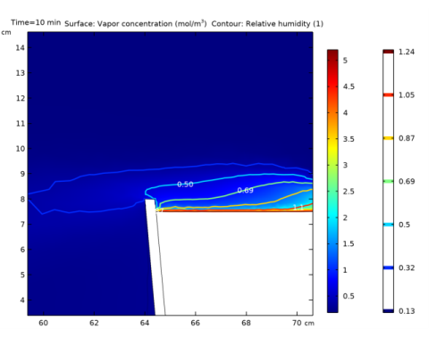
In the Settings window for 2D Plot Group, type Moisture Concentration and Relative Humidity in the Label text field.
3
Locate the Data section. From the Dataset list, choose Cut Plane 1.
4
From the Time (min) list, choose 10.
Surface 1
1
In the Moisture Concentration and Relative Humidity toolbar, click  Surface.
2
In the Settings window for Surface, click Replace Expression in the upper-right corner of the Expression section. From the menu, choose Component 1 (comp1)>Moisture Transport in Air>mt.cv - Vapor concentration - mol/m³.
Moisture Concentration and Relative Humidity
In the Model Builder window, click Moisture Concentration and Relative Humidity.
Contour 1
1
In the Moisture Concentration and Relative Humidity toolbar, click  Contour.
2
In the Settings window for Contour, locate the Expression section.
3
In the Expression text field, type mt.phi.
4
Locate the Levels section. In the Total levels text field, type 7.
5
Locate the Coloring and Style section. From the Contour type list, choose Tube.
6
Select the Radius scale factor check box.
7
8
Select the Level labels check box.
9
In the Precision text field, type 2.
10
From the Label color list, choose White.
11
In the Moisture Concentration and Relative Humidity toolbar, click  Plot.
Use the Zoom Box button in the Graphics window to get a better view of the contour lines.
The relative humidity decreases quickly with the distance to the surface. Due to the high temperature behind the beaker, the relative humidity becomes even lower than 20%.
It is interesting to see how the average temperature decreases with time.
Average Water Temperature
1
In the Results toolbar, click  More Derived Values and choose Average>Volume Average.
2
In the Settings window for Volume Average, type Average Water Temperature in the Label text field.
3
Locate the Data section. From the Dataset list, choose Study 2 : no latent heat source/Solution 3 (sol3).
4
5
Click Replace Expression in the upper-right corner of the Expressions section. From the menu, choose Component 1 (comp1)>Heat Transfer in Moist Air>Temperature>T - Temperature - K.
6
Locate the Expressions section. In the table, enter the following settings:
7
Click  Evaluate.
Table
1
Go to the Table window.
2
Click Table Graph in the window toolbar.
Results
Average Water Temperature over Time
1
In the Model Builder window, under Results click 1D Plot Group 8.
2
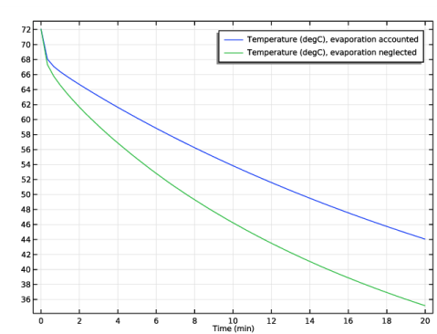
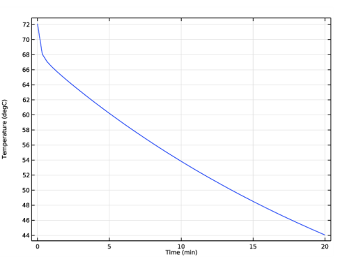
In the Settings window for 1D Plot Group, type Average Water Temperature over Time in the Label text field.
Finally, compute how much water is evaporated in the air.
Amount of Evaporated Water
1
In the Results toolbar, click  More Derived Values and choose Integration>Surface Integration.
2
In the Settings window for Surface Integration, type Amount of Evaporated Water in the Label text field.
3
Locate the Data section. From the Dataset list, choose Study 2 : no latent heat source/Solution 3 (sol3).
4
5
Locate the Expressions section. In the table, enter the following settings:
6
Locate the Data Series Operation section. From the Operation list, choose Integral.
7
Clicknext to  Evaluate, then choose New Table.
Table
1
Go to the Table window.
The factor 2 in the expression is based on the use of a symmetry condition. Within 20 minutes, about 11.2 g of water have been evaporated.
Multiphysics
Repeat the previous steps with a third study that takes latent heat source due to evaporation into account. A comparison with the results returned by Study 2 will then highlight and quantify the cooling effects of evaporation.
Heat and Moisture 2 (ham2)
1
In the Physics toolbar, click  Multiphysics Couplings and choose Domain>Heat and Moisture.
2
Heat and Moisture 1 (ham1)
1
In the Model Builder window, right-click Heat and Moisture 1 (ham1) and choose Disable.
To keep Study 1 and Study 2 in their original states, disable the Heat and Moisture multiphysics coupling feature from their physics trees.
Study 1
Step 1: Wall Distance Initialization
1
In the Model Builder window, under Study 1 click Step 1: Wall Distance Initialization.
2
In the Settings window for Wall Distance Initialization, locate the Physics and Variables Selection section.
3
In the table, clear the Solve for check box for Heat and Moisture 2 (ham2).
Step 2: Stationary
1
In the Model Builder window, click Step 2: Stationary.
2
In the Settings window for Stationary, locate the Physics and Variables Selection section.
3
In the table, clear the Solve for check box for Heat and Moisture 2 (ham2).
Study 2 : no latent heat source
Step 1: Time Dependent
1
In the Model Builder window, under Study 2 : no latent heat source click Step 1: Time Dependent.
2
In the Settings window for Time Dependent, locate the Physics and Variables Selection section.
3
In the table, clear the Solve for check box for Heat and Moisture 2 (ham2).
Add Study
1
In the Home toolbar, click  Add Study to open the Add Study window.
2
Go to the Add Study window.
3
Find the Physics interfaces in study subsection. In the table, clear the Solve check box for Turbulent Flow, Low Re k-ε (spf).
4
Find the Studies subsection. In the Select Study tree, select General Studies>Time Dependent.
5
Click Add Study in the window toolbar.
6
In the Home toolbar, click  Add Study to close the Add Study window.
Study 3 : latent heat source
1
In the Model Builder window, click Study 3.
2
In the Settings window for Study, type Study 3 : latent heat source in the Label text field.
Step 1: Time Dependent
1
In the Model Builder window, click Step 1: Time Dependent.
2
In the Settings window for Time Dependent, locate the Study Settings section.
3
From the Time unit list, choose min.
4
In the Output times text field, type range(0,20[s],20).
5
Locate the Values of Dependent Variables section. Find the Values of variables not solved for subsection. From the Settings list, choose User controlled.
6
From the Method list, choose Solution.
7
From the Study list, choose Study 1, Stationary.
Solution 4 (sol4)
1
In the Study toolbar, click  Show Default Solver.
2
In the Model Builder window, expand the Solution 4 (sol4) node, then click Time-Dependent Solver 1.
3
In the Settings window for Time-Dependent Solver, locate the Time Stepping section.
4
From the Maximum step constraint list, choose Constant.
5
In the Maximum step text field, type 1.
6
Right-click Time-Dependent Solver 1 and choose Fully Coupled.
7
In the Settings window for Fully Coupled, locate the Method and Termination section.
8
From the Jacobian update list, choose On every iteration.
Step 1: Time Dependent
In the Study toolbar, click  Compute.
Results
Temperature (ht) 1
Compute the average temperature of water when evaporation is neglected.
Average Water Temperature 1
1
In the Model Builder window, right-click Average Water Temperature and choose Duplicate.
2
In the Settings window for Volume Average, locate the Data section.
3
From the Dataset list, choose Study 3 : latent heat source/Solution 4 (sol4).
4
Click  Evaluate.
Table
1
Go to the Table window.
2
Click Table Graph in the window toolbar.
Results
Table Graph 1
1
In the Model Builder window, expand the Results>Tables node, then click Results>Average Water Temperature over Time>Table Graph 1.
2
In the Settings window for Table Graph, click to expand the Legends section.
3
Select the Show legends check box.
4
From the Legends list, choose Manual.
5
6
In the Average Water Temperature over Time toolbar, click  Plot.
In this model, evaporation accounts for a decrease of about 10 K at the end of the simulation (see Figure 5).