PDF

Dynamic Wall Heat Exchanger
Introduction
The dynamic wall heat exchanger aims to improve heat transfer in small scale heat exchangers and to reduce pressure drop by using a dynamic wall with an oscillating wave shape. The model is inspired from Ref. 1.
Such deformations of the fluid domain induce mixing of the fluid and reduce the formation of thermal boundary layers. Hence, they increase heat transfer between the walls and the fluid. In addition, the wave shaped deformation induces a pumping effect similar to a peristaltic pumping which compensates the pressure losses.
Model Definition
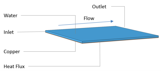
Figure 1 shows the geometry of the heat flux in a static configuration with a flat upper wall. Water is heated as it flows from the inlet to the outlet due to a heat flux at the bottom side of the heat sink. The delivered heat rate at the bottom boundary is set to 125 W.
Figure 1: Geometry and operating conditions of the heat exchanger.
The upper wall of the dynamic wall heat exchanger is deformed to obtained a transient oscillating shape. The upper wall displacement, u, is defined by
(1)
where:
X and Y are the space coordinates on the material frame
t is the time variable
A is the ratio of oscillation amplitude to channel height
fX(X) gives the normalized amplitude of the spatial oscillations in the X direction
ft(t) is the normalized amplitude of the oscillations as a function of time and included a smooth starting effect
N is the number of waves in the channel length direction
L is the channel length
f is the oscillation frequency
Figure 2 shows the shape of the oscillating wall in a cross section parallel to the flow direction after the starting effect.
Figure 2: Oscillating shape of the wall heat exchanger.
Results
In a first step, the performances of the heat exchanger are evaluated for a static configuration. A stationary analysis is computed with no displacement of the upper channel wall.
Figure 3: Temperature distribution in the static heat exchanger.
Figure 3 shows the temperature distribution in the channel in stationary regime where the mass flow rate is 5.5 g/s.
The overall heat transfer coefficient of the heat exchanger is defined as
(2)
and evaluates to about 2,900 W/m² in this application.
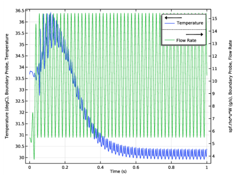
Then, a time dependent analysis is performed where the upper wall displacement is prescribed according to Equation 2, using an oscillation amplitude of 90%. The average outlet temperature and the mass flow rate is monitored during the simulation using probes. As shown in Figure 4, a pseudo-periodic regime is reached after 0.6 s.
Figure 4: Flow rate and outlet temperature variations during the simulation.
As expected, the flow rate increases compared to the static case. The average value over the last period is 10.5 g/s, which is close to twice higher than in the static case.
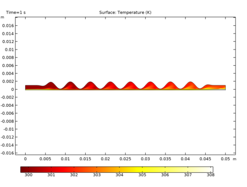
Figure 5 shows the temperature profile in the dynamic wall heat exchanger at time 0.6 s.
Figure 5: Temperature distribution in the dynamic wall heat exchanger.
Finally, the global heat transfer coefficient is estimated using a time average over the last period
(3)
Again, the use of a dynamic wall improves the overall heat rate, equal to 19,000 W/m² with an oscillation amplitude of 90%.
Reference
1. P. Kumar, K. Schmidmayer, F. Topin, and M. Miscevic, “Heat transfer enhancement by dynamic corrugated heat exchanger wall: Numerical study,” Journal of Physics: Conference Series, vol. 745, 2016.
Application Library path: Heat_Transfer_Module/Heat_Exchangers/dynamic_wall_heat_exchanger
Modeling Instructions
From the File menu, choose New.
New
In the New window, click  Model Wizard.
Model Wizard
1
In the Model Wizard window, click  2D.
2
In the Select Physics tree, select Heat Transfer>Conjugate Heat Transfer>Laminar Flow.
3
Click Add.
4
Click  Study.
5
In the Select Study tree, select General Studies>Stationary.
6
Global Definitions
Parameters 1
1
In the Model Builder window, under Global Definitions click Parameters 1.
2
In the Settings window for Parameters, locate the Parameters section.
3
Click  Load from File.
4
Geometry 1
The first domain corresponds to the water channel.
Rectangle 1 (r1)
1
In the Geometry toolbar, click  Rectangle.
2
In the Settings window for Rectangle, locate the Size and Shape section.
3
In the Width text field, type L.
4
In the Height text field, type H.
The second domain corresponds to the copper wall.
Rectangle 2 (r2)
1
In the Geometry toolbar, click  Rectangle.
2
In the Settings window for Rectangle, locate the Size and Shape section.
3
In the Width text field, type L.
4
In the Height text field, type H/5.
5
Locate the Position section. In the y text field, type -H/5.
Definitions
Linear Projection 1 (linproj1)
1
In the Definitions toolbar, click  Nonlocal Couplings and choose Linear Projection.
2
3
In the Settings window for Linear Projection, locate the Source Vertices section.
4
Select the  Activate Selection toggle button for Source vertex 1.
5
6
Select the  Activate Selection toggle button for Source vertex 2.
7
8
Select the  Activate Selection toggle button for Source vertex 3.
9
10
Locate the Destination Vertices section. Select the  Activate Selection toggle button for Destination vertex 1.
11
12
Select the  Activate Selection toggle button for Destination vertex 2.
13
Average 1 (aveop1)
1
In the Definitions toolbar, click  Nonlocal Couplings and choose Average.
2
In the Settings window for Average, locate the Source Selection section.
3
From the Geometric entity level list, choose Boundary.
4
Next, import variables that are needed to define the channel deformation and for postprocessing purposes.
Variables 1
1
In the Model Builder window, right-click Definitions and choose Variables.
2
In the Settings window for Variables, locate the Variables section.
3
Click  Load from File.
4
Add Material
1
In the Home toolbar, click  Add Material to open the Add Material window.
2
Go to the Add Material window.
3
In the tree, select Built-in>Water, liquid.
4
Click  Add to Component 1 (comp1).
5
In the tree, select Built-in>Copper.
6
Click  Add to Component 1 (comp1).
7
In the Home toolbar, click  Add Material to close the Add Material window.
Materials
Copper (mat2)
Select Domain 1 only.
Definitions
Ambient Properties 1 (ampr1)
1
In the Physics toolbar, click  Shared Properties and choose Ambient Properties.
2
In the Settings window for Ambient Properties, locate the Ambient Conditions section.
3
In the Tamb text field, type T0.
Heat Transfer in Solids and Fluids (ht)
Now, define the settings of the Heat Transfer interface.
1
In the Model Builder window, under Component 1 (comp1) click Heat Transfer in Solids and Fluids (ht).
2
In the Settings window for Heat Transfer in Solids and Fluids, locate the Physical Model section.
3
In the dz text field, type W.
4
In the Tref text field, type T0.
Fluid 1
1
In the Model Builder window, under Component 1 (comp1)>Heat Transfer in Solids and Fluids (ht) click Fluid 1.
2
Initial Values 1
1
In the Model Builder window, click Initial Values 1.
2
In the Settings window for Initial Values, locate the Initial Values section.
3
From the T list, choose Ambient temperature (ampr1).
Inflow 1
1
In the Physics toolbar, click  Boundaries and choose Inflow.
2
3
In the Settings window for Inflow, locate the Upstream Properties section.
4
From the Tustr list, choose Ambient temperature (ampr1).
5
Locate the Boundary Selection section. Click  Create Selection.
6
In the Create Selection dialog box, type Inlet in the Selection name text field.
7
Outflow 1
1
In the Physics toolbar, click  Boundaries and choose Outflow.
2
3
In the Settings window for Outflow, locate the Boundary Selection section.
4
Click  Create Selection.
5
In the Create Selection dialog box, type Outlet in the Selection name text field.
6
Heat Flux 1
1
In the Physics toolbar, click  Boundaries and choose Heat Flux.
2
3
In the Settings window for Heat Flux, locate the Heat Flux section.
4
Click the Heat rate button.
5
In the P0 text field, type P0.
Laminar Flow (spf)
The following instructions set the Laminar Flow interface active on the water domain only, and models the flow as incompressible by using a constant density in the simulation. The reference temperature is set in the Heat Transfer interface.
1
In the Model Builder window, under Component 1 (comp1) click Laminar Flow (spf).
2
3
In the Settings window for Laminar Flow, locate the Physical Model section.
4
From the Compressibility list, choose Incompressible flow.
Inlet 1
1
In the Physics toolbar, click  Boundaries and choose Inlet.
2
In the Settings window for Inlet, locate the Boundary Selection section.
3
From the Selection list, choose Inlet.
4
Locate the Boundary Condition section. From the list, choose Pressure.
5
Locate the Pressure Conditions section. In the p0 text field, type Pin.
Outlet 1
1
In the Physics toolbar, click  Boundaries and choose Outlet.
2
In the Settings window for Outlet, locate the Boundary Selection section.
3
From the Selection list, choose Outlet.
Mesh 1
Mapped 1
In the Mesh toolbar, click  Mapped.
Size
1
In the Model Builder window, click Size.
2
In the Settings window for Size, locate the Element Size section.
3
From the Calibrate for list, choose Fluid dynamics.
4
From the Predefined list, choose Extra coarse.
Now, compute the stationary solution for the static configuration of the heat exchanger.
5
In the Home toolbar, click  Compute.
Results
Temperature (ht)
The first default plot shows the temperature profile in the channel (see Figure 3).
Mass Flow Rate, Static Case
1
In the Results toolbar, click  More Derived Values and choose Integration>Line Integration.
2
In the Settings window for Line Integration, type Mass Flow Rate, Static Case in the Label text field.
3
Locate the Selection section. From the Selection list, choose Outlet.
4
Locate the Expressions section. In the table, enter the following settings:
5
Click  Evaluate.
Heat Transfer Coefficient, Static Case
1
In the Results toolbar, click  Global Evaluation.
2
In the Settings window for Global Evaluation, type Heat Transfer Coefficient, Static Case in the Label text field.
3
Click Replace Expression in the upper-right corner of the Expressions section. From the menu, choose Component 1 (comp1)>Definitions>Variables>htc - Global heat transfer coefficient - W/(m²·K).
4
Click  Evaluate.
Definitions
Now, update the model to define the dynamic wall.
Boundary Probe, Temperature
1
In the Definitions toolbar, click  Probes and choose Boundary Probe.
2
In the Settings window for Boundary Probe, type Boundary Probe, Temperature in the Label text field.
3
Locate the Source Selection section. From the Selection list, choose Outlet.
4
Locate the Expression section. From the Table and plot unit list, choose degC.
Boundary Probe, Flow Rate
1
Right-click Boundary Probe, Temperature and choose Duplicate.
2
In the Settings window for Boundary Probe, type Boundary Probe, Flow Rate in the Label text field.
3
Locate the Probe Type section. From the Type list, choose Integral.
4
Locate the Expression section. In the Expression text field, type spf.rho*u*W.
5
In the Table and plot unit field, type g/s.
Prescribed Deformation 1
1
In the Definitions toolbar, click  Moving Mesh and choose Prescribed Deformation.
2
3
In the Settings window for Prescribed Deformation, locate the Prescribed Deformation section.
4
Specify the dx vector as
The Moving Mesh subtree, containing Prescribed Deformation, is only relevant for time-dependent studies. In the next steps, disable Moving Mesh from Study 1 as this is a stationary study, and create a new time-dependent study accounting for moving mesh.
Study 1
Step 1: Stationary
1
In the Model Builder window, under Study 1 click Step 1: Stationary.
2
In the Settings window for Stationary, locate the Physics and Variables Selection section.
3
Select the Modify model configuration for study step check box.
4
In the Physics and variables selection tree, select Component 1 (comp1)>Definitions>Moving Mesh, Controls spatial frame.
5
Click  Disable in Solvers.
6
Click  Control Frame Deformation.
Add Study
1
In the Home toolbar, click  Add Study to open the Add Study window.
2
Go to the Add Study window.
3
Find the Studies subsection. In the Select Study tree, select General Studies>Time Dependent.
4
Click Add Study in the window toolbar.
5
In the Home toolbar, click  Add Study to close the Add Study window.
Study 2
Step 1: Time Dependent
1
In the Settings window for Time Dependent, locate the Study Settings section.
2
In the Output times text field, type range(0,step,end).
3
Click to expand the Values of Dependent Variables section. Find the Initial values of variables solved for subsection. From the Settings list, choose User controlled.
4
From the Method list, choose Solution.
5
From the Study list, choose Study 1, Stationary.
Prescribe a maximum time step to the solver.
Solution 2 (sol2)
1
In the Study toolbar, click  Show Default Solver.
2
In the Model Builder window, expand the Solution 2 (sol2) node, then click Time-Dependent Solver 1.
3
In the Settings window for Time-Dependent Solver, click to expand the Time Stepping section.
4
From the Maximum step constraint list, choose Constant.
5
In the Maximum step text field, type 1/(5*freq).
6
In the Study toolbar, click  Compute.
During the computation, you can visualize how the mass flow rate and average outlet temperature vary in time with the displayed probe plots. Notice that after a number of periods the solution becomes identical over the periods, which indicates that the system has reached a pseudo-stationary state.
Results
Temperature (ht) 1
The first default plot shows the temperature profile in the channel (see Figure 5).
1
In the Settings window for 2D Plot Group, locate the Plot Settings section.
2
From the Frame list, choose Spatial  (x, y, z).
3
Locate the Color Legend section. From the Position list, choose Bottom.
4
In the Temperature (ht) 1 toolbar, click  Plot.
The probe plot can also be displayed by selecting the corresponding node (see Figure 4).
Temperature and Flow Rate
1
In the Model Builder window, under Results click Probe Plot Group 9.
2
In the Settings window for 1D Plot Group, type Temperature and Flow Rate in the Label text field.
Probe Table Graph 1
1
In the Model Builder window, expand the Temperature and Flow Rate node, then click Probe Table Graph 1.
2
In the Settings window for Table Graph, locate the Data section.
3
In the Columns list, select Temperature (degC), Boundary Probe, Temperature.
4
Click to expand the Legends section. From the Legends list, choose Manual.
5
6
7
Click  Delete.
Table Graph 2
1
In the Model Builder window, right-click Temperature and Flow Rate and choose Table Graph.
2
In the Settings window for Table Graph, locate the Data section.
3
From the Table list, choose Probe Table 3.
4
From the Plot columns list, choose Manual.
5
In the Columns list, select spf.rho*u*W (g/s), Boundary Probe, Flow Rate.
6
Locate the Legends section. Select the Show legends check box.
7
From the Legends list, choose Manual.
8
Temperature and Flow Rate
1
In the Model Builder window, click Temperature and Flow Rate.
2
In the Settings window for 1D Plot Group, locate the Plot Settings section.
3
Select the Two y-axes check box.
4
In the table, select the Plot on secondary y-axis check box for Table Graph 2.
5
In the Temperature and Flow Rate toolbar, click  Plot.
Mass Flow Rate, Static Case
Duplicate the two derived values defined in the first study and update them to compute the average over the last period of the flow rate and of the global heat transfer coefficient.
Mass Flow Rate, Dynamic Case
1
In the Model Builder window, right-click Mass Flow Rate, Static Case and choose Duplicate.
2
In the Settings window for Line Integration, type Mass Flow Rate, Dynamic Case in the Label text field.
3
Locate the Data section. From the Dataset list, choose Study 2/Solution 2 (sol2).
4
From the Time selection list, choose Interpolated.
5
In the Times (s) text field, type range(end-1/freq,step,end).
6
Locate the Data Series Operation section. From the Operation list, choose Average.
7
Click  Evaluate.
Heat Transfer Coefficient, Dynamic Case
1
In the Model Builder window, right-click Heat Transfer Coefficient, Static Case and choose Duplicate.
2
In the Settings window for Global Evaluation, type Heat Transfer Coefficient, Dynamic Case in the Label text field.
3
Locate the Data section. From the Dataset list, choose Study 2/Solution 2 (sol2).
4
From the Time selection list, choose Interpolated.
5
In the Times (s) text field, type range(end-1/freq,step,end).
6
Locate the Data Series Operation section. From the Operation list, choose Average.
To create a 3D plot showing both the temperature at the bottom of the heat sink and the fluid velocity, follow the instructions below.
7
Click  Evaluate.
Extrusion 2D 1
1
In the Results toolbar, click  More Datasets and choose Extrusion 2D.
2
In the Settings window for Extrusion 2D, locate the Data section.
3
From the Dataset list, choose Study 2/Solution 2 (sol2).
4
Locate the Extrusion section. In the z maximum text field, type 0.01.
Velocity and Temperature 3D
1
In the Results toolbar, click  3D Plot Group.
2
In the Settings window for 3D Plot Group, type Velocity and Temperature 3D in the Label text field.
3
Locate the Plot Settings section. Clear the Plot dataset edges check box.
Velocity
1
Right-click Velocity and Temperature 3D and choose Surface.
2
In the Settings window for Surface, type Velocity in the Label text field.
3
Locate the Expression section. In the Expression text field, type spf.U.
4
In the Velocity and Temperature 3D toolbar, click  Plot.
Temperature
1
In the Model Builder window, right-click Velocity and Temperature 3D and choose Surface.
2
In the Settings window for Surface, type Temperature in the Label text field.
3
Locate the Expression section. From the Unit list, choose degC.
4
Locate the Coloring and Style section. From the Color table list, choose ThermalLight.
Deformation 1
1
Right-click Temperature and choose Deformation.
2
In the Settings window for Deformation, locate the Expression section.
3
In the x component text field, type 0.
4
In the y component text field, type -0.005.
5
In the z component text field, type 0.
6
Locate the Scale section. Select the Scale factor check box.
7
8
In the Velocity and Temperature 3D toolbar, click  Plot.
Temperature (ht) 1
Finally, create an animation showing the shape of the channel and the temperature distribution over time.
1
In the Model Builder window, click Temperature (ht) 1.
Animation 1
1
In the Temperature (ht) 1 toolbar, click  Animation and choose Player.
2
In the Settings window for Animation, locate the Frames section.
3
From the Frame selection list, choose All.
4
Right-click Animation 1 and choose Play.