Double-Pipe Heat Exchanger

A double-pipe heat exchanger consists of two concentric pipes often performing a U-turn. Due to low costs, it has a large range of applications especially in the chemical process industry. Another advantage is that it can operate at very high pressures. For different scopes, the double-pipe heat exchanger can be stacked in series.

Figure 1: Geometry and concept of the double-pipe heat exchanger.

This tutorial shows how to efficiently model a double-pipe heat exchanger and focuses on preparing the geometry in order to build a suitable mesh manually. In addition, typical postprocessing options are shown.

Model Definition

The concept and basic geometry of the double-pipe heat exchanger is shown in Figure 1. The heat exchanger is made of high tensile steel (Steel AISI 4340). The radii of the concentric pipes are 2.55 cm and 4.8 cm, while the overall length is about 6 m. Due to this high aspect ratio, the mesh has to be carefully handled.

Engine oil at 130°C flows through the outer pipe and is cooled by a transformer oil at 60°C, flowing in countercurrent through the inner pipe to prevent the engine oil from overheating. The material properties of both oils depend on the temperature, and thus the Nonisothermal Flow predefined multiphysics coupling is used.

Flow Regime

To decide whether the flow is laminar or turbulent, estimate the Reynolds number beforehand. The Reynolds number for flows inside a pipe is defined as

where ρ is the density of the fluid, v the typical velocity (taken as the inlet velocity), μ the viscosity, and DH the hydraulic diameter. For the inner pipe, DH is equal to the diameter of the pipe, and for the outer pipe it is the difference between the pipes radii. Adhere to the typical values in Table 1 to evaluate Re.

Table 1: Typical quantities for the Reynolds number.
Quantity	Symbol	Inner pipe	Outer pipe
Density	ρ	850 kg/m3	825 kg/m3
Inlet velocity	v	0.205 m/s	0.09 m/s
Typical length	DH	5.1 cm	1.3 cm
Dynamic viscosity	μ	5·10-3 Pa·s	1·10-3 Pa·s

The Reynolds number for the inner and outer pipe are about 1800 and 1000, respectively. Based on this approximation the Nonisothermal Flow multiphysics coupling in laminar regime is used.

Meanwhile, the densities of the two separated fluids can be considered constant thanks to small temperature variations in each of the inner and outer pipes. Both fluid flows can then be modeled by incompressible formulations.

Boundary conditions

The body of the heat exchanger is modeled as a shell in 3D. This requires special boundary conditions for the flow and heat transport equations. The interior wall condition separates the pipes and applies a no slip condition for the flow on both sides.

To account for the in-plane heat flux in the shell, the boundary condition is applied. This boundary condition simulates heat transfer in thin shell structures. Here, the shell is made of steel with a 7 mm thickness.

The inlet boundary condition applies a laminar inflow profile at the pipe’s ends. Refer to the Heat Transfer Module User’s Guide for more information about the settings for this boundary condition. The engine oil enters the outer pipe at 130 °C and with an average velocity of 0.09 m/s. The transformer oil enters the inner pipe at 60 °C and with an average velocity of 0.205 m/s.

The outlets are connected to pipes of same diameter. For this configuration, the option in the feature is particularly suited.

At exterior boundaries, the model assumes thermal insulation because the losses to the outside are considered negligible.

Results and Discussion

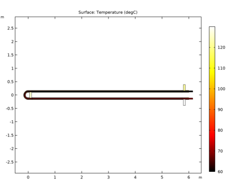
Figure 2 shows the temperature distribution along the center plane. The transformer oil is heated up by 9°C to 69°C while the engine oil is cooled by 7°C to 123°C.

Figure 2: Temperature field in the central plane, zoomed at inlet and outlet regions.

The next plot shows the velocity field.

Figure 3: Velocity magnitude inside the pipes, zoomed at inlet and outlet regions.

The calculated pressure drops are close to 155 Pa for the inner pipe and slightly less than 1400 Pa for the outer pipe.

The equivalent heat transfer coefficient describes the heat exchanger’s performance. It is given by

(1)

where P is the total exchanged power and A is the surface area of the interface between the two fluids. In this model the value of heq is about 41 W/(m2·K).

Notes About the COMSOL Implementation

Setting up of the Nonisothermal Flow multiphysics coupling is straightforward according to the descriptions above. Due to the high nonlinearity in the model, initial values affect convergence. It is sufficient to set the initial temperature to (Thot + Tcold) ⁄ 2. Furthermore, the fluids that are considered incompressible would have densities equal to a reference value, ρ(Tref), taken at a reference temperature of Tcold at inner pipes and Thot at outer pipes.

In this tutorial, using a physics-induced mesh leads to a large number of mesh elements. The long straight parts of the pipes can be meshed more efficiently with a swept mesh without losing accuracy. Therefore, the geometry needs to be divided into three parts: the U-turn, the straight parts, and the inlets/outlets (see Figure 4). The Modeling Instructions section below contains the steps for preparing and meshing the geometry as well as the postprocessing part.

Figure 4: Geometry of the double-pipe heat exchanger divided into three parts.

Heat_Transfer_Module/Heat_Exchangers/double_pipe_heat_exchanger

Reference

1. H. S. Lee, Thermal Design, John Wiley & Sons, 2010.

Modeling Instructions

Root

From the menu, choose .

Browse to the model’s Application Libraries folder and double-click the file double_pipe_heat_exchanger_preset.mph.

Component 1 (comp1)

To evaluate the equivalent heat transfer coefficient after the simulation, define a nonlocal integration coupling over the interior walls.

Definitions (comp1)

Average Over Interior Wall

In the toolbar, click

and choose .

In the window for , type Average Over Interior Wall in the text field.

Locate the section. From the list, choose .

From the list, choose .

The physics-controlled mesh is satisfying for fluid flow models with boundary layers at all no-slip boundaries. The gradient along the pipes is expected to be very low compared to the gradient perpendicular to the pipes cross-sections. Hence, a swept mesh is an appropriate choice for meshing the straight part of the pipes, reducing the computational costs while keeping accuracy. Before it is applicable, the geometry needs to be prepared to have the straight part of the pipes as separate domains. This can be done by partitioning the geometry with work planes. The predefined selections in ensure that the physical settings still apply to the correct entities, even after the partitioning operations.

Geometry 1

Work Plane 1 (wp1)

In the toolbar, click

In the window for , locate the section.

From the list, choose .

On the object , select Boundary 27 only.

It might be easier to select the correct boundary by using the window. To open this window, in the toolbar click and choose . (If you are running the cross-platform desktop, you find in the main menu.)