PDF

Radiation in a Cavity
Introduction
The following example shows how to build and solve a radiative heat transfer problem using the Heat Transfer with Surface-to-Surface Radiation interface. This example’s simple geometry allows a comparison of results from COMSOL Multiphysics with a theoretical solution.
Model Definition
The geometry consists of three rectangles with lengths 3 m, 4 m, and 5 m, and all have a width of 1 m. The rectangles are situated such that they form a triangular cavity (see Figure 1).
Figure 1: Three domains form a triangular cavity to study heat radiation.
The rectangles are made of copper, which is a good thermal conductor, and they transfer heat internally by conduction. Further, the three inner boundaries that form the cavity can exchange heat only by means of surface-to-surface radiation. The surface emissivities are ε1 = 0.4 on the bottom boundary, ε2 = 0.6 on the vertical boundary, and ε3 = 0.8 on the inclined boundary.
The system holds the temperature on the (outer) lower boundary at T1 = 300 K. Further, the system experiences an inward heat flux of q2 = 2000 W/m2 on the outer boundary of the vertical rectangle and q3 = 1000 W/m2 on the outer boundary of the tilted one. All remaining outer boundaries are insulated.
This example examines the steady state of the cavity’s interior boundaries. Specifically, you know the value of the heat flux on the inclined and vertical boundaries, and you want to find the temperature along these boundaries. Conversely, you know the temperature of the bottom boundary and want to determine the heat flux that leaves through it.
Results and Discussion
Figure 2 shows the temperature field resulting from a simulation. If you run the model as described later in this section you can see from the color display that the temperatures are fairly constant within the three rectangles. The theoretical results predict that a heat flux Q1 = −11,000 W/m leaves the cavity through the bottom boundary, that the vertical boundary has a temperature of T2 = 641 K, and that the inclined boundary has a temperature of T3 = 600 K. The results obtained are very close to these theoretical values. The section Comparing Results with Theory provides more details on the verification of these results.
Figure 2: Temperature as a function of position.
Figure 3 details the temperature distribution along the inclined boundary of the cavity. Note that while the temperature is not constant, it varies by only a few percent. The lowest temperature appears on the lower-left, and the highest temperature is on the right, which seems reasonable because that portion of the boundary is located adjacent to the vertical boundary, which has the highest inward heat flux.
Figure 3: Temperature distribution along the inclined boundary of the cavity.
Figure 3 plots the radiosity along the inclined boundary (in other words, the total heat flux that leaves the boundary into the cavity). The radiosity is the sum of the heat flux the boundary emits plus the heat flux it reflects.
Figure 4: Radiosity along the inclined boundary of the cavity.
Like temperature, the radiosity is fairly constant along the boundary. The small variations have roughly the same distribution as the temperature in Figure 3.
Comparing Results with Theory
As mentioned at the start of this section, you can compare the results from this tutorial to theoretical values, which are based on the sketch in Figure 5 and whose theory appears in the section “Enclosures with More Than Two Surfaces” in Ref. 1.
Figure 5: Problem sketch for theoretical analysis of radiation in a triangular cavity.
The theoretical model considers only the three boundaries that form the cavity. On these boundaries, the model either holds the temperature at a constant value or specifies a heat flux. Note that this approach differs somewhat from the model, which sets temperatures and heat fluxes on the rectangles’ outer boundaries.
The COMSOL Multiphysics model shows that the temperatures and heat fluxes are nearly equal on the inner and outer boundaries of the rectangles. Therefore, the COMSOL Multiphysics and the theoretical model show good agreement.
Using the notation from Figure 5 with the same assumptions as for the model, you obtain the following lengths and emissivities:
L1 = 4 m, ε1 = 0.4
L2 = 3 m, ε2 = 0.6
L3 = 5 m, ε3 = 0.8
The boundary conditions define either the temperature or the heat flux on each boundary. Now apply the same boundary conditions as in the problem where you set values for T1, Q2, and Q3. You must, however, make a small adjustment for T1 because the theoretical configuration sets it on the outer boundary and not on the cavity side. T1 is therefore slightly higher than 300 K in the theoretical analysis:
You describe the heat flux from a boundary with the following two equations:
For a triangular cavity, the following equation gives the view factor between surface i and surface j:
Substituting this expression for the view factor into the second equation for the heat fluxes results in a linear system of six equations. The six unknowns for this particular problem are J1, J2, J3, Q1, T2, and T3, and you would like to compare the three last to those from the solution. Solving the linear system yields the following values: Q1 = −11,000 W/m, T2 = 641 K, and T3 = 600 K.
To compare these results with the model, you must find the total heat flux through the cavity’s bottom (horizontal) boundary and also calculate the average temperatures on the other two boundaries.
The following table compares the results from COMSOL Multiphysics with the theoretical values:
Q1
T2
T3
The differences are quite small. Also note that the theoretical model includes some simplifications. For example, it assumes that heat fluxes and temperatures are constant along each boundary. It also assumes a constant view factor for each pair of boundaries, whereas COMSOL Multiphysics computes a local view factor at each point of the cavity.
Reference
1. A. Bejan, Heat Transfer, John Wiley & Sons, 1993.
Application Library path: Heat_Transfer_Module/Verification_Examples/cavity_radiation
Modeling Instructions
From the File menu, choose New.
New
In the New window, click  Model Wizard.
Model Wizard
1
In the Model Wizard window, click  2D.
2
In the Select Physics tree, select Heat Transfer>Radiation>Heat Transfer with Surface-to-Surface Radiation.
3
Click Add.
4
Click  Study.
5
In the Select Study tree, select General Studies>Stationary.
6
Geometry 1
The geometry consists of three rectangles positioned such that they create a triangular cavity.
Rectangle 1 (r1)
1
In the Geometry toolbar, click  Rectangle.
2
In the Settings window for Rectangle, locate the Size and Shape section.
3
In the Width text field, type 4.
4
Locate the Position section. In the y text field, type -1.
Rectangle 2 (r2)
1
In the Geometry toolbar, click  Rectangle.
2
In the Settings window for Rectangle, locate the Size and Shape section.
3
In the Height text field, type 3.
4
Locate the Position section. In the x text field, type 4.
Rectangle 3 (r3)
1
In the Geometry toolbar, click  Rectangle.
2
In the Settings window for Rectangle, locate the Size and Shape section.
3
In the Width text field, type 5.
4
Locate the Rotation Angle section. In the Rotation text field, type atan(3/4)[rad].
Form Union (fin)
1
In the Model Builder window, under Component 1 (comp1)>Geometry 1 click Form Union (fin).
2
In the Settings window for Form Union/Assembly, locate the Form Union/Assembly section.
3
From the Action list, choose Form an assembly.
4
In the Geometry toolbar, click  Build All.
5
Click the  Zoom Extents button in the Graphics toolbar.
This completes the geometry modeling stage.
Materials
Copper
1
In the Materials toolbar, click  Blank Material.
2
In the Settings window for Material, type Copper in the Label text field.
3
Locate the Material Contents section. In the table, enter the following settings:
Heat Transfer in Solids (ht)
Initial Values 1
1
In the Model Builder window, under Component 1 (comp1)>Heat Transfer in Solids (ht) click Initial Values 1.
2
In the Settings window for Initial Values, locate the Initial Values section.
3
In the T text field, type 300.
Next, define the boundary conditions.
Heat Flux 1
1
In the Physics toolbar, click  Boundaries and choose Heat Flux.
2
3
In the Settings window for Heat Flux, locate the Heat Flux section.
4
In the q0 text field, type 1000.
Heat Flux 2
1
In the Physics toolbar, click  Boundaries and choose Heat Flux.
2
3
In the Settings window for Heat Flux, locate the Heat Flux section.
4
In the q0 text field, type 2000.
Temperature 1
1
In the Physics toolbar, click  Boundaries and choose Temperature.
2
3
In the Settings window for Temperature, locate the Temperature section.
4
In the T0 text field, type 300.
Surface-to-Surface Radiation (rad)
1
In the Model Builder window, under Component 1 (comp1) click Surface-to-Surface Radiation (rad).
2
Diffuse Surface 1
1
In the Model Builder window, under Component 1 (comp1)>Surface-to-Surface Radiation (rad) click Diffuse Surface 1.
2
In the Settings window for Diffuse Surface, locate the Ambient section.
3
Find the Ambient temperature subsection. In the Tamb text field, type 300.
4
Locate the Surface Emissivity section. From the ε list, choose User defined. In the associated text field, type 0.8.
When the Heat Transfer with Surface-to-Surface Radiation multiphysics coupling is added the default domain opacity is set to From heat transfer interface which means that the solid domains are opaque by default while the fluid domains are transparent by default. You can override these default settings by adding one or multiple Opacity node(s) under the Surface-to-Surface Radiation interface.
Diffuse Surface 2
1
In the Physics toolbar, click  Boundaries and choose Diffuse Surface.
2
3
In the Settings window for Diffuse Surface, locate the Ambient section.
4
Find the Ambient temperature subsection. In the Tamb text field, type 300.
5
Locate the Surface Emissivity section. From the ε list, choose User defined. In the associated text field, type 0.4.
Diffuse Surface 3
1
In the Physics toolbar, click  Boundaries and choose Diffuse Surface.
2
3
In the Settings window for Diffuse Surface, locate the Ambient section.
4
Find the Ambient temperature subsection. In the Tamb text field, type 300.
5
Locate the Surface Emissivity section. From the ε list, choose User defined. In the associated text field, type 0.6.
Mesh 1
Edge 1
1
In the Mesh toolbar, click  Edge.
2
In the Settings window for Edge, locate the Boundary Selection section.
3
From the Geometric entity level list, choose Entire geometry.
Size 1
1
Right-click Edge 1 and choose Size.
2
In the Settings window for Size, locate the Geometric Entity Selection section.
3
From the Geometric entity level list, choose Boundary.
4
5
Locate the Element Size section. Click the Custom button.
6
Locate the Element Size Parameters section. Select the Maximum element size check box.
7
Size 2
1
In the Model Builder window, right-click Edge 1 and choose Size.
2
In the Settings window for Size, locate the Geometric Entity Selection section.
3
From the Geometric entity level list, choose Point.
4
5
Locate the Element Size section. Click the Custom button.
6
Locate the Element Size Parameters section. Select the Maximum element size check box.
7
8
Click  Build Selected.
Free Triangular 1
1
In the Mesh toolbar, click  Free Triangular.
2
In the Settings window for Free Triangular, click to expand the Tessellation section.
3
From the Method list, choose Advancing front.
4
In the Model Builder window, right-click Mesh 1 and choose Build All.
The complete mesh consists of roughly 2,700 elements.
Study 1
1
In the Home toolbar, click  Compute.
The computation takes a few seconds.
Results
Temperature (ht)
The first default plot shows the temperature field; compare with Figure 2.
The two additional default plots visualize the temperature field isothermal contours, and the radiosity on the boundaries.
Add a 1D plot for the temperature field on the inclined boundary (Figure 3).
Temperature Profile vs. Arc Length
1
In the Home toolbar, click  Add Plot Group and choose 1D Plot Group.
2
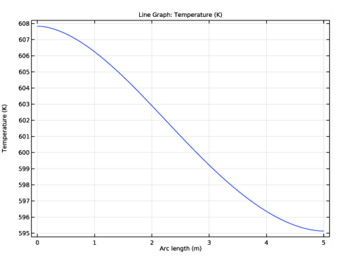
In the Settings window for 1D Plot Group, type Temperature Profile vs. Arc Length in the Label text field.
Line Graph 1
1
In the Temperature Profile vs. Arc Length toolbar, click  Line Graph.
2
3
In the Temperature Profile vs. Arc Length toolbar, click  Plot.
Temperature Profile vs. Arc Length
Add another 1D plot showing the radiosity on the inclined boundary (Figure 4).
Surface Radiosity Profile vs. Arc Length
1
In the Model Builder window, right-click Temperature Profile vs. Arc Length and choose Duplicate.
2
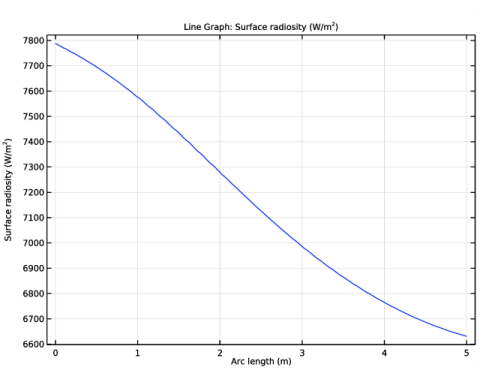
In the Settings window for 1D Plot Group, type Surface Radiosity Profile vs. Arc Length in the Label text field.
Line Graph 1
1
In the Model Builder window, expand the Surface Radiosity Profile vs. Arc Length node, then click Line Graph 1.
2
In the Settings window for Line Graph, click Replace Expression in the upper-right corner of the y-Axis Data section. From the menu, choose Component 1 (comp1)>Surface-to-Surface Radiation>Surface radiosity>rad.J - Surface radiosity - W/m².
3
In the Surface Radiosity Profile vs. Arc Length toolbar, click  Plot.
Determine the conductive heat flux through the cavity’s bottom boundary as follows.
Line Integration 1
1
In the Results toolbar, click  More Derived Values and choose Integration>Line Integration.
2
3
In the Settings window for Line Integration, click Replace Expression in the upper-right corner of the Expressions section. From the menu, choose Component 1 (comp1)>Heat Transfer in Solids>Boundary fluxes>ht.ndflux - Normal conductive heat flux - W/m².
4
Click  Evaluate.
Table
1
Go to the Table window.
The result displayed in the Table window should be approximately -11,000 W/m.
Next, find the mean temperature on the vertical boundary of the cavity.
Results
Line Integration 2
1
In the Results toolbar, click  More Derived Values and choose Integration>Line Integration.
2
3
In the Settings window for Line Integration, locate the Expressions section.
4
5
Click  Evaluate.
Table
1
Go to the Table window.
The resulting temperature, read from the table, should be approximately 645 K.
Finally, evaluate the mean temperature on inclined boundary of the cavity.
Results
Line Integration 3
1
In the Results toolbar, click  More Derived Values and choose Integration>Line Integration.
2
3
In the Settings window for Line Integration, locate the Expressions section.
4
5
Click  Evaluate.
Table
1
Go to the Table window.
The resulting temperature, read from the table, should be approximately 600 K.