PDF

Fluid-Structure Interaction in Aluminum Extrusion
Introduction
Out of all metals, the most frequently extruded is aluminum. Aluminum extrusion entails using a hydraulic ram to squeeze an aluminum bar through a die. This process will form the metal into a particular shape. Extruded aluminum is used in many manufacturing applications, such as building components for example. In massive forming processes like rolling or extrusion, metal alloys are deformed in a hot solid state with material flowing under ideally plastic conditions. Such processes can be simulated effectively using computational fluid dynamics, where the material is considered as a fluid with a very high viscosity that depends on velocity and temperature. Internal friction of the moving material acts as a heat source, so that the heat transfer equations are fully coupled with those ruling the fluid dynamics part. This approach is especially advantageous when large deformations are involved.
This model is adapted from a benchmark study in Ref. 1. The original benchmark solves a thermal-structural coupling, because it is common practice in the simulation of such processes to use specific finite element codes that have the capability to couple the structural equations with heat transfer. The alternative scheme discussed here couples non-Newtonian flow with heat transfer equations. In addition, because it is useful to know the stress in the die due to fluid pressure and thermal loads, the model adds a structural mechanics analysis.
The die design is courtesy of Compes S.p.A., while the die geometry, boundary conditions, and experimental data are taken from Ref. 1.
Note: This application requires the Heat Transfer Module and the Structural Mechanics Module. In addition, it uses the Material Library.
Model Definition
The model considers steady-state conditions, assuming a billet of infinite length flowing through the die. In the actual process, the billet is pushed by the ram through the die and its volume is continuously reducing.
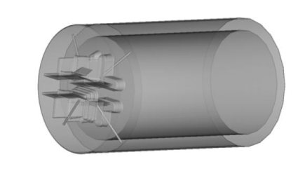
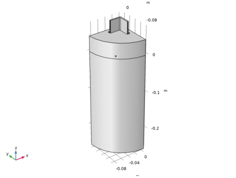
Figure 1 shows the original complete geometry with four different profiles. To have a model with reasonable dimensions, consider only a quarter of the original geometry. The simplification involved in neglecting the differences between the four profiles does not affect the numerical scheme proposed. Figure 2 shows the resulting model geometry.
Figure 1: Original benchmark geometry.
Figure 2: Quarter of the original geometry considered in the model.
Material Properties
The documentation for the benchmark model (Ref. 1) serves as the data source for properties of the two main materials: AISI steel for the die and the container (the ram is not considered here) and aluminum for the billet.
Structural Analysis
Because only the steel part is active in the structural analysis, consider a simple linear elastic behavior where the elastic properties are those of the material H11 mod (AISI 610) that can be found in the COMSOL Multiphysics Material Library.
Heat Transfer Analysis
The benchmark model uses the following properties for aluminum and steel:
kal
ρal
Cpal
2.94 N/(mm2·K)/ρal
kfe
ρfe
Cpfe
4.63 N/(mm2·K)/ρfe
Non-Newtonian Flow
The properties of the aluminum were experimentally determined and then checked using literature data for the same alloy and surface state. However the benchmark proposes an experimental constitutive law, suited for the structural mechanics codes usually used to simulate such processes, in the form of the flow stress data. For this model this requires a recalculation of the constitutive law to derive a general expression for the viscosity. The equivalent von Mises stress, σeqv, can be defined in terms of the total contraction of the deviatoric stress tensor as
or, using where is the strain rate and η is the viscosity, as
(1)
Introducing the equivalent strain rate
Equation 1 can be expressed as
The strain rate tensor is defined as (Ref. 2)
The shear rate is defined as
so that
The flow rule
states that plastic yielding occurs if the equivalent stress, σeqv, reaches the flow stress, κf. The viscosity is defined as (see Ref. 2 for further details)
The organizers of the benchmark propose specific flow-stress data expressed in terms of a generalized Zener-Hollomon function
where A = 2.39·108 s1, n = 2.976, α = 0.052 MPa1, and
with 153 kJ/mol and R = 8.314 J/(K·mol).
Sources, Initial Conditions, and Boundary Conditions
Structural Analysis
Because the model geometry is a quarter of the actual geometry, use symmetric boundary conditions for the two orthogonal planes. On the external surfaces of the die, apply roller boundary conditions because in reality other dies, not considered here, are present to increase the system’s stiffness.
The main loads are the thermal loads from the heat transfer analysis and the total stress from the fluid dynamics analysis.
Heat Transfer Analysis
For the billet, use a volumetric heat source related to the viscous heating effect.
The external temperature of the ram and the die is held constant at 450 °C (723 K). The ambient temperature is 25 °C (298 K). For the heat exchange between aluminum and steel, use the heat transfer coefficient of 11 N/(s·mm·K). Also consider convective heat exchange with air outside the profiles with a fixed convective heat transfer coefficient of 15 W/(m2·K).
Apply initial temperatures as given in the following table:
380 °C (653 K)
450 °C (723 K)
460 °C (733 K)
404 °C (677 K)
Non-Newtonian Flow
At the inlet, the ram moves with a constant velocity of 0.5 mm/s. Impose this boundary condition by simply applying a constant inlet velocity. At the outlet, a normal stress condition with zero external pressure applies. On the surfaces placed on the two symmetry planes, use symmetric conditions. Finally, apply slip boundary conditions on the boundaries placed outside the profile.
Results and Discussion
The general response of the proposed numerical scheme, especially in the zone of the profile, is in good accordance with the experience of the designers. A comparison between the available experimental data and the numerical results of the simulation shows good agreement.
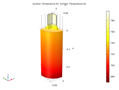
On the basis of the results from the simulation, the engineer can improve the preliminary die design by adjusting relevant physical parameters and operating conditions. For this purpose, the volume plot in Figure 3 showing the temperature field inside the profile gives important information. Furthermore, the combined streamline and slice plot in Figure 4 reveals any imbalances in the velocity field that could result in a crooked profile. A proper design should also ensure that different parts of the profile travel at the same speed. Figure 5 shows the von Mises equivalent stress in the steel part considering the thermal load and the pressure load due to the presence of the fluid.
Figure 3: Temperature distribution in the billet.
Figure 4: Velocity field and streamlines at the profile section.
Figure 5: Equivalent von Mises stress distribution in the container.
References
1. M. Schikorra, L. Donati, L. Tomesani, and A.E. Tekkaya, “The Extrusion Benchmark 2007,” Proceedings of the Extrusion Workshop 2007 and 2nd Extrusion Benchmark Conference, Bologna, Italy, http://diemtech.ing.unibo.it/extrusion07.
2. E.D. Schmitter, “Modelling massive forming processes with thermally coupled fluid dynamics,” Proceedings of the COMSOL Multiphysics User's Conference 2005 Frankfurt, Frankfurt, Germany.
Application Library path: Heat_Transfer_Module/Thermal_Processing/aluminum_extrusion_fsi
Modeling Instructions
From the File menu, choose New.
New
In the New window, click  Model Wizard.
Model Wizard
1
In the Model Wizard window, click  3D.
2
In the Select Physics tree, select Heat Transfer>Conjugate Heat Transfer>Laminar Flow.
3
Click Add.
4
In the Select Physics tree, select Structural Mechanics>Solid Mechanics (solid).
5
Click Add.
6
Click  Study.
7
In the Select Study tree, select General Studies>Stationary.
8
Geometry 1
Import 1 (imp1)
1
In the Home toolbar, click  Import.
2
In the Settings window for Import, locate the Import section.
3
Click Browse.
4
5
Click Import.
6
Click the  Zoom Extents button in the Graphics toolbar.
The imported geometry contains narrow face regions, which are not necessary for this model and will increase the number of elements significantly. Add a Remove Details feature to remove these details.
Remove Details 1 (rmd1)
1
In the Geometry toolbar, click  Remove Details.
2
Click  Build All.
You should now see the following geometry.
Global Definitions
Parameters 1
1
In the Model Builder window, under Global Definitions click Parameters 1.
2
In the Settings window for Parameters, locate the Parameters section.
3
Definitions
Variables 1
1
In the Home toolbar, click  Variables and choose Local Variables.
2
In the Settings window for Variables, locate the Variables section.
3
Create the selections to simplify the model specification.
Outside
1
In the Definitions toolbar, click  Explicit.
2
In the Settings window for Explicit, type Outside in the Label text field.
3
Locate the Input Entities section. From the Geometric entity level list, choose Boundary.
4
For more convenience in selecting these boundaries, you can click the Paste Selection button and paste the above numbers.
Interior
1
In the Definitions toolbar, click  Explicit.
2
In the Settings window for Explicit, type Interior in the Label text field.
3
Locate the Input Entities section. From the Geometric entity level list, choose Boundary.
4
Before creating the materials for the model, specify the fluid and solid domains. Using this information, the software can detect which material properties are needed.
Heat Transfer in Solids and Fluids (ht)
Fluid 1
1
In the Model Builder window, under Component 1 (comp1)>Heat Transfer in Solids and Fluids (ht) click Fluid 1.
2
3
In the Settings window for Fluid, locate the Domain Selection section.
4
Click  Create Selection.
5
In the Create Selection dialog box, type Billet in the Selection name text field.
6
Laminar Flow (spf)
1
In the Model Builder window, under Component 1 (comp1) click Laminar Flow (spf).
2
In the Settings window for Laminar Flow, locate the Physical Model section.
3
From the Compressibility list, choose Incompressible flow.
4
Locate the Domain Selection section. From the Selection list, choose Billet.
Solid Mechanics (solid)
1
In the Model Builder window, under Component 1 (comp1) click Solid Mechanics (solid).
2
In the Settings window for Solid Mechanics, locate the Domain Selection section.
3
Click  Clear Selection.
4
Now, define the material for each domain.
Add Material
1
In the Home toolbar, click  Add Material to open the Add Material window.
2
Go to the Add Material window.
3
In the tree, select Material Library>Tool Steels>H11 mod (AISI 610)>H11 mod (AISI 610) [solid].
4
Click Add to Component in the window toolbar.
5
In the Home toolbar, click  Add Material to close the Add Material window.
Materials
H11 mod (AISI 610) [solid] (mat1)
1
2
In the Settings window for Material, locate the Material Contents section.
3
The heat capacity is not used since it does not enter in the stationary heat transfer equation for solids without translational movement. The heat capacity is only provided for completeness in case you want to extend the model to perform transient simulations.
Billet
1
In the Materials toolbar, click  Blank Material.
2
In the Settings window for Material, type Billet in the Label text field.
3
Locate the Geometric Entity Selection section. From the Selection list, choose Billet.
4
Locate the Material Contents section. In the table, enter the following settings:
H11 mod (AISI 610) [solid] 1 (mat3)
1
In the Model Builder window, under Component 1 (comp1)>Materials right-click H11 mod (AISI 610) [solid] (mat1) and choose Duplicate.
2
In the Settings window for Material, locate the Geometric Entity Selection section.
3
From the Geometric entity level list, choose Boundary.
4
From the Selection list, choose Interior.
Now, define the volume reference temperature in the solid domains. This temperature is used by materials to define the density in solids for both the Heat Transfer and Solid Mechanics interfaces, and by the Thermal Expansion feature as the zero strain reference.
Definitions
Model Input 1
1
In the Physics toolbar, click  Shared Properties and choose Model Input.
2
3
In the Settings window for Model Input, locate the Definition section.
4
Click  Select Quantity.
5
In the Physical Quantity dialog box, type temperature in the text field.
6
Click  Filter.
7
In the tree, select General>Volume reference temperature (K).
8
9
In the Settings window for Model Input, locate the Definition section.
10
This value overrides the value defined under Default Model Inputs for the selected domain.
Model Input 2
1
In the Physics toolbar, click  Shared Properties and choose Model Input.
2
3
In the Settings window for Model Input, locate the Definition section.
4
Click  Select Quantity.
5
In the Physical Quantity dialog box, select General>Volume reference temperature (K) in the tree.
6
7
In the Settings window for Model Input, locate the Definition section.
8
With the materials defined, you can set up the remaining physics of the model.
Laminar Flow (spf)
In the current model, the viscosity in the fluid flow part is large, which implies that the model is diffusion dominated. Pseudo time stepping works poorly for this model because it is based on the scale of the convective flux.
1
Click the  Show More Options button in the Model Builder toolbar.
2
In the Show More Options dialog box, in the tree, select the check box for the node Physics>Advanced Physics Options.
3
4
In the Model Builder window, click Laminar Flow (spf).
5
In the Settings window for Laminar Flow, click to expand the Advanced Settings section.
6
Find the Pseudo time stepping subsection. From the Use pseudo time stepping for stationary equation form list, choose Off.
Initial Values 1
1
In the Model Builder window, under Component 1 (comp1)>Laminar Flow (spf) click Initial Values 1.
2
In the Settings window for Initial Values, locate the Initial Values section.
3
In the p text field, type P_init.
Symmetry 1
1
In the Physics toolbar, click  Boundaries and choose Symmetry.
2
Inlet 1
1
In the Physics toolbar, click  Boundaries and choose Inlet.
2
3
In the Settings window for Inlet, locate the Velocity section.
4
Click the Velocity field button.
5
Specify the u0 vector as
Wall 2
1
In the Physics toolbar, click  Boundaries and choose Wall.
2
In the Settings window for Wall, locate the Boundary Selection section.
3
From the Selection list, choose Outside.
4
Locate the Boundary Condition section. From the Wall condition list, choose Slip.
Outlet 1
1
In the Physics toolbar, click  Boundaries and choose Outlet.
2
3
In the Settings window for Outlet, locate the Pressure Conditions section.
4
In the p0 text field, type P_init.
Heat Transfer in Solids and Fluids (ht)
Initial Values 1
1
In the Model Builder window, under Component 1 (comp1)>Heat Transfer in Solids and Fluids (ht) click Initial Values 1.
2
In the Settings window for Initial Values, locate the Initial Values section.
3
In the T text field, type T_container.
Temperature 1
1
In the Physics toolbar, click  Boundaries and choose Temperature.
2
3
In the Settings window for Temperature, locate the Temperature section.
4
In the T0 text field, type T_container.
Heat Flux 1
1
In the Physics toolbar, click  Boundaries and choose Heat Flux.
2
3
In the Settings window for Heat Flux, locate the Heat Flux section.
4
Click the Convective heat flux button.
5
In the h text field, type Heat_alfe.
6
In the Text text field, type T_ram.
Heat Flux 2
1
In the Physics toolbar, click  Boundaries and choose Heat Flux.
2
In the Settings window for Heat Flux, locate the Boundary Selection section.
3
From the Selection list, choose Outside.
4
Locate the Heat Flux section. Click the Convective heat flux button.
5
In the h text field, type H_conv.
6
In the Text text field, type T_air.
Outflow 1
1
In the Physics toolbar, click  Boundaries and choose Outflow.
2
Thin Layer 1
1
In the Physics toolbar, click  Boundaries and choose Thin Layer.
2
In the Settings window for Thin Layer, locate the Boundary Selection section.
3
From the Selection list, choose Interior.
4
Locate the Layer Model section. From the Specify list, choose Thermal resistance.
5
Locate the Heat Conduction section. In the Rs text field, type 1/Heat_alfe.
Materials
H11 mod (AISI 610) [solid] 1 (mat3)
1
In the Model Builder window, under Component 1 (comp1)>Materials click H11 mod (AISI 610) [solid] 1 (mat3).
2
In the Settings window for Material, locate the Material Contents section.
3
Solid Mechanics (solid)
For faster convergence use linear elements. You can always refine the solution using the default quadratic elements.
1
In the Model Builder window, under Component 1 (comp1) click Solid Mechanics (solid).
2
In the Settings window for Solid Mechanics, click to expand the Discretization section.
3
From the Displacement field list, choose Linear.
Linear Elastic Material 1
Both Young’s modulus and Poisson’s ratio are temperature dependent. Follow these steps to verify that the temperature is defined by the Heat Transfer interface.
1
In the Model Builder window, under Component 1 (comp1)>Solid Mechanics (solid) click Linear Elastic Material 1.
2
In the Settings window for Linear Elastic Material, locate the Model Input section.
3
Click  Go to Source for the Temperature (T).
Global Definitions
Default Model Inputs
Locate the Browse Model Inputs section. The icon column of the table under Model input contributions shows that it is the Heat Transfer interface that defines the temperature in the solid and fluid domains and on the thin-layer boundaries.
Solid Mechanics (solid)
Roller 1
1
In the Physics toolbar, click  Boundaries and choose Roller.
2
Symmetry 1
1
In the Physics toolbar, click  Boundaries and choose Symmetry.
2
Multiphysics
Fluid-Structure Interaction 1 (fsi1)
1
In the Physics toolbar, click  Multiphysics Couplings and choose Boundary>Fluid-Structure Interaction.
2
In the Settings window for Fluid-Structure Interaction, locate the Boundary Selection section.
3
From the Selection list, choose All boundaries.
Thermal Expansion 1 (te1)
1
In the Physics toolbar, click  Multiphysics Couplings and choose Domain>Thermal Expansion.
2
Mesh 1
Free Triangular 1
1
In the Mesh toolbar, click  Boundary and choose Free Triangular.
2
Size 1
1
Right-click Free Triangular 1 and choose Size.
2
In the Settings window for Size, locate the Element Size section.
3
Click the Custom button.
4
Locate the Element Size Parameters section. Select the Maximum element size check box.
5
6
Select the Curvature factor check box.
7
8
Click  Build Selected.
Swept 1
1
In the Mesh toolbar, click  Swept.
2
In the Settings window for Swept, locate the Domain Selection section.
3
From the Geometric entity level list, choose Domain.
4
Distribution 1
1
Right-click Swept 1 and choose Distribution.
2
In the Settings window for Distribution, locate the Distribution section.
3
In the Number of elements text field, type 24.
4
Click  Build All.
Free Tetrahedral 1
In the Mesh toolbar, click  Free Tetrahedral.
Size 1
1
Right-click Free Tetrahedral 1 and choose Size.
2
In the Settings window for Size, locate the Element Size section.
3
Click the Custom button.
4
Locate the Element Size Parameters section. Select the Maximum element size check box.
5
Size 2
1
In the Model Builder window, right-click Free Tetrahedral 1 and choose Size.
2
In the Settings window for Size, locate the Geometric Entity Selection section.
3
From the Geometric entity level list, choose Boundary.
4
5
Locate the Element Size section. Click the Custom button.
6
Locate the Element Size Parameters section. Select the Maximum element size check box.
7
Size 3
1
Right-click Free Tetrahedral 1 and choose Size.
2
In the Settings window for Size, locate the Geometric Entity Selection section.
3
From the Geometric entity level list, choose Domain.
4
5
Locate the Element Size section. Click the Custom button.
6
Locate the Element Size Parameters section. Select the Minimum element size check box.
7
Size
1
In the Model Builder window, click Size.
2
In the Settings window for Size, locate the Element Size section.
3
From the Predefined list, choose Finer.
4
Click  Build All.
You should now see the following meshed geometry.
Study 1
Step 1: Stationary
Use two stationary study steps. Solve first for the fluid dynamics and heat transfer to determine the thermal load and the pressure load and then for the structural mechanics.
1
In the Model Builder window, under Study 1 click Step 1: Stationary.
2
In the Settings window for Stationary, locate the Physics and Variables Selection section.
3
In the table, clear the Solve for check box for Solid Mechanics (solid).
4
In the table, clear the Solve for check boxes for Fluid-Structure Interaction 1 (fsi1) and Thermal Expansion 1 (te1).
Stationary 2
1
In the Study toolbar, click  Study Steps and choose Stationary>Stationary.
2
In the Settings window for Stationary, locate the Physics and Variables Selection section.
3
In the table, clear the Solve for check boxes for Heat Transfer in Solids and Fluids (ht) and Laminar Flow (spf).
4
In the table, clear the Solve for check box for Nonisothermal Flow 1 (nitf1).
For the structural analysis, use a memory efficient iterative solver to make it possible to solve the problem also on computers with limited memory.
Solution 1 (sol1)
1
In the Study toolbar, click  Show Default Solver.
2
In the Model Builder window, expand the Solution 1 (sol1) node.
3
In the Model Builder window, expand the Study 1>Solver Configurations>Solution 1 (sol1)>Stationary Solver 2 node.
4
Right-click Stationary Solver 2 and choose Iterative.
5
In the Study toolbar, click  Compute.
Results
Temperature (ht)
The first default plot shows the temperature (Figure 3).
1
In the Settings window for 3D Plot Group, locate the Data section.
2
From the Dataset list, choose Exterior Walls.
3
In the Temperature (ht) toolbar, click  Plot.
Modify the third default plot to see the velocity field and streamlines at the profile section (Figure 4).
Study 1/Solution Store 1 (sol2)
In the Model Builder window, expand the Results>Datasets node, then click Study 1/Solution Store 1 (sol2).
Selection
1
In the Results toolbar, click  Attributes and choose Selection.
2
In the Settings window for Selection, locate the Geometric Entity Selection section.
3
From the Geometric entity level list, choose Domain.
4
From the Selection list, choose Billet.
Velocity (spf)
1
In the Model Builder window, click Velocity (spf).
2
In the Settings window for 3D Plot Group, locate the Data section.
3
From the Dataset list, choose Study 1/Solution Store 1 (sol2).
Slice
1
In the Model Builder window, expand the Velocity (spf) node, then click Slice.
2
In the Settings window for Slice, locate the Plane Data section.
3
From the Plane list, choose xy-planes.
4
From the Entry method list, choose Coordinates.
5
In the z-coordinates text field, type 0.0151.
6
In the Velocity (spf) toolbar, click  Plot.
Velocity (spf)
In the Model Builder window, click Velocity (spf).
Streamline 1
1
In the Velocity (spf) toolbar, click  Streamline.
2
In the Settings window for Streamline, click Replace Expression in the upper-right corner of the Expression section. From the menu, choose Component 1 (comp1)>Laminar Flow>Velocity and pressure>u,v,w - Velocity field (spatial frame).
3
Locate the Streamline Positioning section. From the Positioning list, choose Magnitude controlled.
4
In the Min distance text field, type 0.01.
5
In the Max distance text field, type 0.1.
6
Locate the Coloring and Style section. Find the Line style subsection. From the Type list, choose Ribbon.
7
In the Width expression text field, type 0.001.
8
Select the Width scale factor check box.
9
Find the Point style subsection. From the Type list, choose Arrow.
10
Select the Number of arrows check box.
11
12
Click to expand the Inherit Style section.
Color Expression 1
1
In the Velocity (spf) toolbar, click  Color Expression.
2
In the Settings window for Color Expression, click Replace Expression in the upper-right corner of the Expression section. From the menu, choose Component 1 (comp1)>Laminar Flow>Velocity and pressure>spf.U - Velocity magnitude - m/s.
Streamline 1
1
In the Model Builder window, click Streamline 1.
2
In the Settings window for Streamline, locate the Inherit Style section.
3
From the Plot list, choose Slice.
4
In the Velocity (spf) toolbar, click  Plot.
To get a better view, rotate the geometry in the Graphics window. You can preserve a view for a plot by creating a View feature node as follows:
5
Click the  Show More Options button in the Model Builder toolbar.
6
In the Show More Options dialog box, in the tree, select the check box for the node Results>Views.
7
View 3D 3
1
In the Model Builder window, right-click Views and choose View 3D.
2
Use the Graphics toolbox to get a satisfying view.
3
In the Settings window for View 3D, locate the View section.
4
Select the Lock camera check box.
Next, apply the view to the velocity plot.
Velocity (spf)
1
In the Model Builder window, click Velocity (spf).
2
In the Settings window for 3D Plot Group, locate the Plot Settings section.
3
From the View list, choose View 3D 3.
4
In the Velocity (spf) toolbar, click  Plot.
For a clearer visualization, you can duplicate this plot group and remove the geometry edges and the velocity slice, and add instead a temperature surface at the outside part.
Velocity and Outside Temperature
1
Right-click Velocity (spf) and choose Duplicate.
2
In the Settings window for 3D Plot Group, type Velocity and Outside Temperature in the Label text field.
3
In the Model Builder window, expand the Velocity and Outside Temperature node.
4
Right-click Velocity and Outside Temperature and choose Move Up.
5
Right-click Velocity and Outside Temperature and choose Move Up.
Slice
In the Model Builder window, right-click Slice and choose Delete.
Surface 2
1
In the Results toolbar, click  More Datasets and choose Surface.
2
Velocity and Outside Temperature
In the Model Builder window, click Velocity and Outside Temperature.
Surface 1
1
In the Velocity and Outside Temperature toolbar, click  Surface.
2
In the Settings window for Surface, locate the Data section.
3
From the Dataset list, choose Surface 2.
4
Locate the Coloring and Style section. From the Color table list, choose ThermalLight.
Velocity and Outside Temperature
1
In the Model Builder window, click Velocity and Outside Temperature.
2
In the Settings window for 3D Plot Group, locate the Color Legend section.
3
From the Position list, choose Right double.
4
Locate the Plot Settings section. Clear the Plot dataset edges check box.
5
In the Velocity and Outside Temperature toolbar, click  Plot.
Stress (solid)
The last plot shows the von Mises stress and deformation distribution in the container. To reproduce the Figure 5, apply the View 3D 2.
1
In the Model Builder window, click Stress (solid).
2
In the Settings window for 3D Plot Group, locate the Plot Settings section.
3
From the View list, choose View 3D 3.
Surface 1
1
In the Model Builder window, expand the Stress (solid) node, then click Surface 1.
2
In the Settings window for Surface, locate the Expression section.
3
From the Unit list, choose GPa.
4
In the Stress (solid) toolbar, click  Plot.