PDF

Tunnel Excavation
Introduction
This example studies the behavior of soil during a tunnel excavation. The surface settlement and the width of the plastic region around the tunnel are important parameters required to predict the reinforcements that are required during the excavation. This verification example is adapted from Ref. 1 and Ref. 2.
In order to calculate in-situ stresses, use two studies. In the first study compute the stress state of the soil before the excavation of the tunnel. In the second study compute the elastoplastic behavior once the soil is removed. This requires incorporation of the stress response calculated in the first study. The soil removal is modeled using the activation feature in the linear elastic material model.
In order to speed up the calculation consider the soil in the first step as elastic, and in the second step, add the Drucker-Prager soil plasticity model. The example is solved in 2D plane strain.
Model Definition
The geometry consists of a soil layer that is 45 m deep and 90 m wide. A tunnel of 10 m in diameter is placed at the symmetry axis, 20 m below the surface. A bed rock, 45 m below the surface, constrains the displacement in the vertical direction, and a roller boundary is used to model the infinite extension of the soil in the lateral direction.
Figure 1: Dimensions and boundary conditions for the tunnel excavation example.
Soil Properties
The soil properties are adapted from Ref. 2.
Young’s modulus, E = 12 MPa and Poisson’s ratio ν = 0.495.
Cohesion c = 130 kPa and angle of internal friction φ = 30 degrees.
Constraints and Loads
Add a Gravity node to account for gravity effects.
Results and Discussion
Figure 2 shows the stress distribution due to gravity. The roller and symmetry boundaries create a linear vertical variation of the stress.
Figure 2: The von Mises stress in the soil layer before excavation of the tunnel.
Figure 3 shows the stress distribution after excavating the tunnel. Note the increase in the equivalent stress around the tunnel.
Figure 3: The von Mises stress in the soil layer after excavation of the tunnel.
In the second step, besides removing the tunnel domain, a soil plasticity feature is included. In Figure 4, the region that experience plastic deformation is shown.
Figure 4: Plastic deformation in the zone near the tunnel after the excavation.
The horizontal displacement and the settlement of the top surface due to the excavation is shown in Figure 5 and Figure 6.
Figure 5: The horizontal displacement at the top surface.
Figure 6: The surface settlement.
References
1. D. Potts and L. Zdravkovic, Finite Element Analysis in Geotechnical Engineering, Thomas Telford Publishing, 2001.
2. H. Schweiger, “Results from Numerical Benchmark Exercises in Geotechnics,” Proc. 5th European Conference on Numerical Methods in Geotechnical Engineering, pp. 305–314, 2002.
Application Library path: Geomechanics_Module/Soil/tunnel_excavation
Modeling Instructions
From the File menu, choose New.
New
In the New window, click  Model Wizard.
Model Wizard
1
In the Model Wizard window, click  2D.
2
In the Select Physics tree, select Structural Mechanics>Solid Mechanics (solid).
3
Click Add.
4
Click  Study.
5
In the Select Study tree, select General Studies>Stationary.
6
Geometry 1
Rectangle 1 (r1)
1
In the Geometry toolbar, click  Rectangle.
2
In the Settings window for Rectangle, locate the Size and Shape section.
3
In the Width text field, type 90.
4
In the Height text field, type 45.
5
Locate the Position section. In the y text field, type -45.
6
Click  Build Selected.
Circle 1 (c1)
1
In the Geometry toolbar, click  Circle.
2
In the Settings window for Circle, locate the Size and Shape section.
3
In the Radius text field, type 5.
4
In the Sector angle text field, type 180.
5
Locate the Position section. In the y text field, type -20.
6
Locate the Rotation Angle section. In the Rotation text field, type 270.
7
Click  Build Selected.
Form Union (fin)
1
In the Model Builder window, click Form Union (fin).
2
In the Settings window for Form Union/Assembly, click  Build Selected.
Use the full geometry and a linear elastic material in the first step.
Solid Mechanics (solid)
Linear Elastic Material 1
Since in this example, the Poisson’s ratio is 0.495, use a mixed formulation to avoid locking effects.
1
In the Model Builder window, under Component 1 (comp1)>Solid Mechanics (solid) click Linear Elastic Material 1.
2
In the Settings window for Linear Elastic Material, locate the Linear Elastic Material section.
3
From the Use mixed formulation list, choose Pressure formulation.
Symmetry 1
1
In the Physics toolbar, click  Boundaries and choose Symmetry.
2
Fixed Constraint 1
1
In the Physics toolbar, click  Boundaries and choose Fixed Constraint.
2
Roller 1
1
In the Physics toolbar, click  Boundaries and choose Roller.
2
Gravity 1
1
In the Physics toolbar, click  Domains and choose Gravity.
2
In the Settings window for Gravity, locate the Domain Selection section.
3
From the Selection list, choose All domains.
Linear Elastic Material 1
In the Model Builder window, click Linear Elastic Material 1.
Soil Plasticity 1
1
In the Physics toolbar, click  Attributes and choose Soil Plasticity.
2
In the Settings window for Soil Plasticity, locate the Soil Plasticity section.
3
Select the Match to Mohr-Coulomb criterion check box.
Add an Initial Stress and Strain node and enable it only in the second study in order to get in-situ stresses due to gravity.
Linear Elastic Material 1
In the Model Builder window, click Linear Elastic Material 1.
Initial Stress and Strain 1
1
In the Physics toolbar, click  Attributes and choose Initial Stress and Strain.
2
In the Settings window for Initial Stress and Strain, locate the Initial Stress and Strain section.
3
In the S0 table, enter the following settings:
Add an Activation node to the linear elastic material in order to model the soil removal. The activation expression set to zero in order to deactivate the material. The elastic stiffness of the soil material is multiplied by activation scale factor.
Linear Elastic Material 1
In the Model Builder window, click Linear Elastic Material 1.
Activation 1
1
In the Physics toolbar, click  Attributes and choose Activation.
2
3
In the Settings window for Activation, locate the Activation section.
4
In the Activation scale factor text field, type 1e-9.
Materials
Material 1 (mat1)
1
In the Model Builder window, under Component 1 (comp1) right-click Materials and choose Blank Material.
2
In the Settings window for Material, locate the Material Contents section.
3
Mesh 1
Free Triangular 1
In the Mesh toolbar, click  Free Triangular.
Size
1
In the Model Builder window, click Size.
2
In the Settings window for Size, locate the Element Size section.
3
From the Predefined list, choose Finer.
Distribution 1
1
In the Model Builder window, right-click Free Triangular 1 and choose Distribution.
2
3
In the Settings window for Distribution, locate the Distribution section.
4
In the Number of elements text field, type 12.
5
Click  Build All.
Use two stationary studies. The first one is used to compute the in-situ stresses. The second study is used to compute the elastoplastic deformation due to the excavation of the tunnel.
Study: Before Excavation
1
In the Model Builder window, click Study 1.
2
In the Settings window for Study, type Study: Before Excavation in the Label text field.
Step 1: Stationary
1
In the Model Builder window, under Study: Before Excavation click Step 1: Stationary.
2
In the Settings window for Stationary, locate the Physics and Variables Selection section.
3
Select the Modify model configuration for study step check box.
4
In the Physics and variables selection tree, select Component 1 (comp1)>Solid Mechanics (solid)>Linear Elastic Material 1>Soil Plasticity 1, Component 1 (comp1)>Solid Mechanics (solid)>Linear Elastic Material 1>Initial Stress and Strain 1, and Component 1 (comp1)>Solid Mechanics (solid)>Linear Elastic Material 1>Activation 1.
5
Click  Disable.
Add Study
1
In the Home toolbar, click  Add Study to open the Add Study window.
2
Go to the Add Study window.
3
Find the Studies subsection. In the Select Study tree, select General Studies>Stationary.
4
Click Add Study in the window toolbar.
5
In the Home toolbar, click  Add Study to close the Add Study window.
Study: After Excavation
1
In the Model Builder window, click Study 2.
2
In the Settings window for Study, type Study: After Excavation in the Label text field.
Study: Before Excavation
In the Home toolbar, click  Compute.
Study: After Excavation
Click  Compute.
Results
Stress: Before Excavation
1
In the Model Builder window, under Results click Stress (solid).
2
In the Settings window for 2D Plot Group, type Stress: Before Excavation in the Label text field.
Surface 1
In the Model Builder window, expand the Stress: Before Excavation node.
Deformation
1
In the Model Builder window, expand the Surface 1 node, then click Deformation.
2
In the Settings window for Deformation, locate the Scale section.
3
Select the Scale factor check box.
4
5
In the Stress: Before Excavation toolbar, click  Plot.
6
Click the  Zoom Extents button in the Graphics toolbar.
The second default plot shows the von Mises stress in the soil after the tunnel excavation.
Stress: After Excavation
1
In the Model Builder window, expand the Results>Stress (solid) 1 node, then click Stress (solid) 1.
2
In the Settings window for 2D Plot Group, type Stress: After Excavation in the Label text field.
Deformation
1
In the Model Builder window, expand the Results>Stress: After Excavation>Surface 1 node, then click Deformation.
2
In the Settings window for Deformation, locate the Scale section.
3
Select the Scale factor check box.
4
Filter 1
1
In the Model Builder window, click Filter 1.
2
In the Settings window for Filter, locate the Element Selection section.
3
From the Element nodes to fulfill expression list, choose All.
4
In the Stress: After Excavation toolbar, click  Plot.
5
Click the  Zoom Extents button in the Graphics toolbar.
Plastic Region: After Excavation
Use this plot group to show the plastic zone after excavation of the tunnel.
1
In the Model Builder window, under Results click Equivalent Plastic Strain (solid).
2
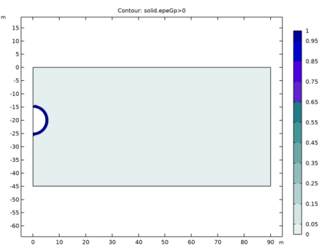
In the Settings window for 2D Plot Group, type Plastic Region: After Excavation in the Label text field.
Contour 1
1
In the Model Builder window, expand the Plastic Region: After Excavation node, then click Contour 1.
2
In the Settings window for Contour, locate the Expression section.
3
In the Expression text field, type solid.epeGp>0.
This is a boolean expression which is 1 in the plastic region and 0 elsewhere.
4
Clear the Description check box.
Deformation 1
1
Right-click Contour 1 and choose Deformation.
2
In the Settings window for Deformation, locate the Scale section.
3
Select the Scale factor check box.
4
5
In the Plastic Region: After Excavation toolbar, click  Plot.
6
Click the  Zoom Extents button in the Graphics toolbar.
Plastic Region: After Excavation
1
In the Model Builder window, click Plastic Region: After Excavation.
2
In the Settings window for 2D Plot Group, click to expand the Selection section.
3
From the Geometric entity level list, choose Domain.
4
5
In the Plastic Region: After Excavation toolbar, click  Plot.
Horizontal Displacement: After Excavation
1
In the Home toolbar, click  Add Plot Group and choose 1D Plot Group.
2
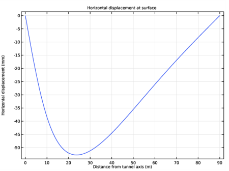
In the Settings window for 1D Plot Group, type Horizontal Displacement: After Excavation in the Label text field.
3
Locate the Data section. From the Dataset list, choose Study: After Excavation/Solution 2 (sol2).
4
Click to expand the Title section. From the Title type list, choose Manual.
5
In the Title text area, type Horizontal displacement at surface.
6
Locate the Plot Settings section. Select the x-axis label check box.
7
In the associated text field, type Distance from tunnel axis (m).
8
Select the y-axis label check box.
9
In the associated text field, type Horizontal displacement (mm).
Line Graph 1
1
Right-click Horizontal Displacement: After Excavation and choose Line Graph.
2
3
In the Settings window for Line Graph, locate the y-Axis Data section.
4
In the Expression text field, type u.
5
From the Unit list, choose mm.
6
In the Horizontal Displacement: After Excavation toolbar, click  Plot.
Vertical Displacement: After Excavation
1
In the Model Builder window, right-click Horizontal Displacement: After Excavation and choose Duplicate.
2
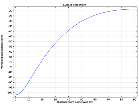
In the Settings window for 1D Plot Group, type Vertical Displacement: After Excavation in the Label text field.
3
Locate the Title section. In the Title text area, type Surface settlement.
4
Locate the Plot Settings section. In the y-axis label text field, type Vertical displacement (mm).
Line Graph 1
1
In the Model Builder window, expand the Vertical Displacement: After Excavation node, then click Line Graph 1.
2
In the Settings window for Line Graph, locate the y-Axis Data section.
3
In the Expression text field, type v.
4
In the Vertical Displacement: After Excavation toolbar, click  Plot.