|
|
|
|
•
|
|
•
|
|
•
|
|
•
|
|
•
|
|
•
|
|
•
|
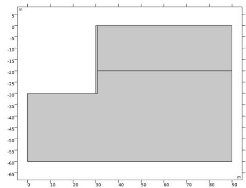
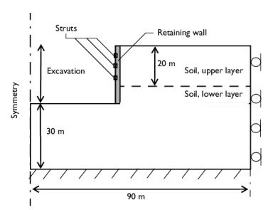
The in-situ stresses account for the local stress prior excavating. You can define a different value in the vertical and horizontal directions. The horizontal in-situ stress, X_stress, is also used on the boundary load applied to the retaining wall.
|
|
•
|
The struts are active after a maximum horizontal deflection is reached. Use a ramp function to restrict the allowed wall deflection U_max to 25 mm, and to supply the axial force that the struts apply to the wall.
|
|
•
|
The axial stiffness of the struts is estimated from their cross sectional area A, the length l, and the material Young’s modulus E as
|
|
1
|
|
2
|
|
3
|
Click Add.
|
|
4
|
Click
|
|
5
|
|
6
|
Click
|
|
1
|
|
2
|
|
1
|
|
2
|
|
3
|
|
4
|
|
5
|
|
6
|
|
1
|
|
2
|
|
3
|
|
4
|
|
5
|
|
6
|
|
7
|
|
1
|
|
2
|
|
3
|
|
4
|
|
5
|
|
6
|
|
1
|
|
2
|
Click in the Graphics window and then press Ctrl+A to select both objects.
|
|
3
|
|
1
|
|
2
|
|
3
|
|
4
|
|
5
|
|
6
|
|
1
|
|
2
|
|
3
|
|
4
|
|
5
|
|
6
|
|
7
|
|
1
|
|
2
|
Select the object uni1 only.
|
|
3
|
|
4
|
|
5
|
|
6
|
|
7
|
|
1
|
|
2
|
|
3
|
|
4
|
|
5
|
|
6
|
|
1
|
|
2
|
|
3
|
|
4
|
|
5
|
|
6
|
|
7
|
|
8
|
|
9
|
|
1
|
|
2
|
|
3
|
|
4
|
|
5
|
|
6
|
|
7
|
|
8
|
|
9
|
|
1
|
|
2
|
|
3
|
|
4
|
|
5
|
|
6
|
|
7
|
|
8
|
|
9
|
|
1
|
|
2
|
|
3
|
|
1
|
|
2
|
|
3
|
|
4
|
|
5
|
|
1
|
|
2
|
|
3
|
|
1
|
|
2
|
|
3
|
|
1
|
|
2
|
|
3
|
|
4
|
|
5
|
|
6
|
Click OK.
|
|
7
|
|
8
|
|
9
|
|
10
|
|
1
|
|
2
|
|
3
|
|
4
|
|
5
|
|
6
|
|
7
|
|
1
|
|
2
|
|
3
|
|
1
|
|
2
|
|
3
|
From the list, choose Diagonal.
|
|
4
|
|
1
|
|
1
|
|
1
|
|
1
|
|
3
|
|
4
|
|
5
|
|
1
|
|
2
|
|
3
|
|
4
|
|
5
|
|
1
|
|
3
|
|
4
|
|
1
|
|
3
|
|
4
|
|
1
|
|
2
|
|
4
|
|
5
|
|
1
|
|
2
|
|
4
|
|
5
|
|
1
|
|
2
|
|
4
|
|
5
|
|
1
|
In the Model Builder window, under Component 1 (comp1) right-click Materials and choose Blank Material.
|
|
2
|
|
3
|
|
4
|
|
6
|
|
1
|
|
2
|
|
4
|
|
1
|
|
2
|
|
4
|
|
1
|
|
2
|
|
3
|
|
1
|
|
2
|
|
3
|
|
4
|
|
1
|
|
2
|
|
3
|
|
4
|
|
5
|
Click OK.
|
|
6
|
|
7
|
|
1
|
|
2
|
|
3
|
|
1
|
|
3
|
|
4
|
|
1
|
|
3
|
|
4
|
|
1
|
|
3
|
|
4
|
|
5
|
|
6
|
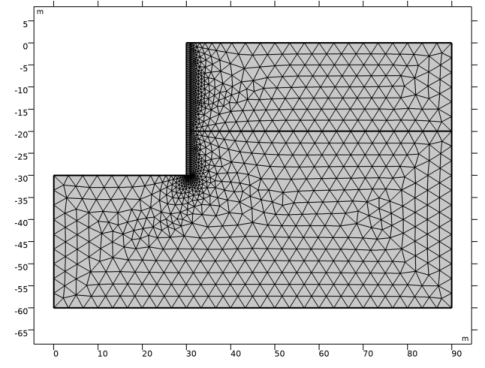
Click the Zoom Box button In the Graphics toolbar and then use the mouse to zoom in on the contact zone where the mesh is the densest.
|
|
1
|
|
2
|
|
3
|
|
4
|
Click
|
|
1
|
|
2
|
|
3
|
In the Model Builder window, expand the Study 1>Solver Configurations>Solution 1 (sol1)>Stationary Solver 1 node, then click Parametric 1.
|
|
4
|
|
5
|
|
6
|
|
7
|
|
8
|
|
9
|
|
1
|
|
1
|
|
2
|
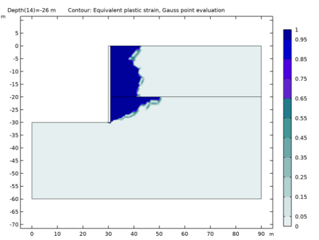
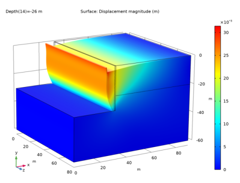
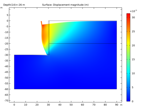
In the Settings window for Surface, click Replace Expression in the upper-right corner of the Expression section. From the menu, choose Component 1 (comp1)>Solid Mechanics>Displacement>solid.disp - Displacement magnitude - m.
|
|
3
|
|
4
|
|
1
|
|
2
|
|
1
|
|
2
|
|
3
|
|
4
|
|
1
|
|
2
|
|
3
|
|
4
|
|
5
|
|
6
|
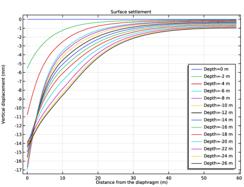
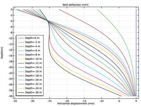
In the associated text field, type Horizontal displacement (mm).
|
|
7
|
|
8
|
In the associated text field, type Depth(m).
|
|
9
|
|
1
|
|
2
|
|
3
|
|
4
|
|
5
|
|
6
|
|
7
|
|
8
|
|
9
|
|
10
|
|
1
|
|
2
|
|
3
|
|
4
|
|
5
|
|
6
|
In the associated text field, type Distance from the diaphragm (m).
|
|
7
|
|
8
|
In the associated text field, type Vertical displacement (mm).
|
|
9
|
|
1
|
|
3
|
|
4
|
|
5
|
|
6
|
|
7
|
|
8
|
|
1
|
|
2
|
|
3
|
|
1
|
|
2
|
|
1
|
|
2
|
|
3
|